Home
Syllabus
Homework
Notes
Announcements
Links

Economics 301
Intermediate Macroeconomics

Production Function

Winter 2000

Last updated: January 25, 2000

Note: These notes are preliminary and incomplete and they are not guaranteed to be free of errors. Please let me know if you find typos or other errors. 

The Production Function

The aggregate production function for the economy is assumed to take the form

Y = A·F(K, N)

where

• Y = real GDP
• A = index of overall productivity in the economy
• K = amount of capital input (measured in physical units or in $ value) in the economy
• N = number of workers employed in the economy

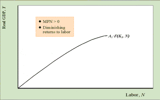
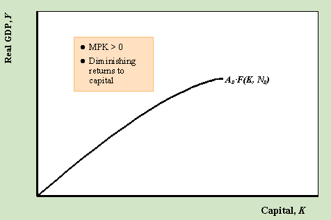
Assumptions concerning the shape of F(K, N)

• Marginal product of labor, MNP, is positive and diminishing ( MPN = DY/DN holding everything else fixed)

The graph above shows the production function as a function of N holding A and K fixed.

• Marginal product of capital, MPK, is positive and diminishing (MPK = DY/DK holding everything else fixed)

The graph above shows the production function as a function of K holding A and N fixed.

Example: Cobb-Douglas constant returns to scale production function

Y = A·K^aN^1-a , 0 < a < 1

where

• a = share of income received by owners of capital
• 1 - a = share of income received by labor

Note: Constant returns to scale means that if we double all inputs to the production function then output exactly doubles.  To see that the Cobb-Douglas exhibits this property, note that

A·(2K)^a(2N)^1-a   = A·2^a2^1-aK^aN^1-a   = 2A·K^aN^1-a  = 2Y

For US data, from the national income and product accounts, we know that labor's share of income is about 0.7 which implies that for the US 1-a = 0.7 and a = 0.3.

A Medium-run Assumption

The production function shows how real GDP, Y, is determined over some fixed time period like a quarter or a year. Over this time period it is assumed that capital stock, K, and the level of overall productivity, A, is held fixed whereas it is assumed that the amount of labor can vary. That is, over the assumed time period, firms in the economy cannot easily alter the amount of capital they use (i.e. buildings, equipment etc.) but they can easily vary the amount of labor that they hire. Similarly, it is assumed that productivity does not change very quickly.  Given, these assumptions we can represent the production function as

Y = A₀F(K₀, N)

where the subscript "0" indicates that the level of productivity is fixed at the amount A₀ and the level of capital is fixed at the amount K₀. The unsubscripted variable, N, is allowed to vary.

Moving Along vs. Shifting Curves

Moving along the production function

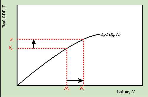
As N increases from N₀ to N₁ output increases from Y₀ to Y₁ as we move along the production function.

Shifting the production function: An increase in productivity

When the index of productivity increases from A₀ to A₁, holding everything else fixed, the production function shifts up. Then for a given amount of labor, N₀, the amount of output produced in the economy increases from Y₀ to Y₁.

Shifting the production function: An increase in the stock of capital

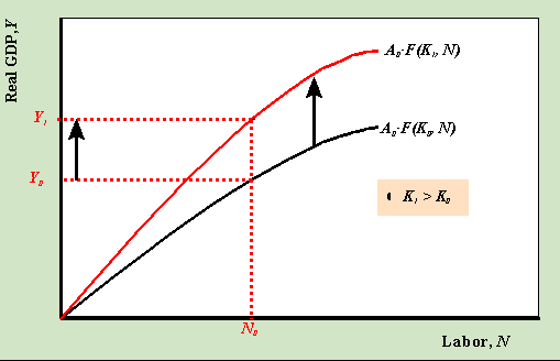
When the capital stock increases from K₀ to K₁, holding everything else fixed, the production function shifts up. Then for a given amount of labor, N₀, the amount of output produced in the economy increases from Y₀ to Y₁.