Last updated:
February 14, 2000
Note: These notes are preliminary and incomplete
and they are not guaranteed to be free of errors. Please let me know if
you find typos or other errors.
Consider the economy initially in general equilibrium with r* = 5% and full
employment output Y*. The vertical line labeled FE represents full
employment output and is equivalent to the long-run aggregate supply
(LRAS) curve. Recall, in general equilibrium the labor market is in
equilibrium, the goods market is in equilibrium (aggregate demand = aggregate supply) and
the money market is in equilibrium. The initial price level is given by P0.

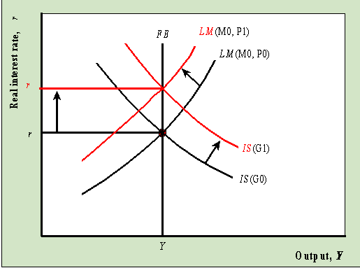
Suppose the government increases its purchases of goods and services from G0
to G1. This increases the aggregate demand for goods and the IS curve
shifts up and to the right. The level of demand is determined by the intersection between
IS and LM and this is denoted Yd. At the higher level of government
spending the aggregate demand for goods is greater than the aggregate supply of goods, Y*.
Firms will see their inventory of goods fall and they will respond by increasing prices.
Also, workers will bargain for higher nominal wages to keep their real wage constant. As
overall prices and wages rise, the LM curve will shift up and to the left and the real
interest rate will rise. As r increases, interest sensitive spending (consumption
and investment) falls as we move along the IS curve toward the new general equilibrium at r
= 8%. At the new equilibrium, output is again Y* but the real interest rate and
the price level are higher. Also, the higher amount of government spending has crowded out
some private consumption and investment expenditure due to the higher real interest rate.
The end result of the increased level of government spending is no increase in real output
but the composition of demand has changed: more government spending and less private
spending.
Consider the economy initially in general equilibrium with r* = 5% and full
employment output Y*. Recall, in general equilibrium the labor market is in
equilibrium, the goods market is in equilibrium (aggregate demand = aggregate supply) and
the money market is in equilibrium. The initial price level is given by P0.

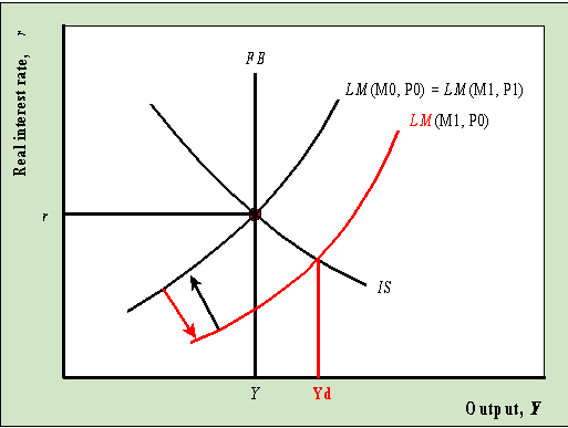
Now suppose the Fed increases the nominal money supply, through an open market purchase
of government bonds, from M0 to M1. This shifts
the LM curve down and to the right and increases the demand for goods by putting downward
pressure on the real interest rate. The level of demand is determined by the intersection
between IS and LM and this is denoted Yd. At the higher level of real
balances the aggregate demand for goods is greater than the aggregate supply of goods, Y*.
Firms will see their inventory of goods fall and they will respond by increasing prices.
Workers react to the increase in prices by bargaining for higher nominal wages to keep
their real wage constant. As overall prices and wage rise, the LM curve will shift up and
to the left reversing the downward pressure on the real interest rate. Prices rise so that
the LM curve shifts right back to where it was initially. The expansionary monetary policy
in this example is completely neutral on the real economy: the increase in M has caused no
change in the equilibrium values of the real variables Y, r, w
(real wage).
The higher money supply has increased the price level and the level of nominal wages and
has caused a brief spurt of inflation.
Consider the economy initially in general equilibrium with r* = 5% and full
employment output Y*. Recall, in general equilibrium the labor market is in
equilibrium, the goods market is in equilibrium (aggregate demand = aggregate supply) and
the money market is in equilibrium. The initial price level is given by P0.

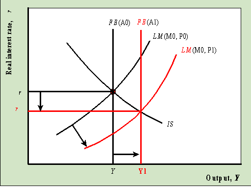
Suppose that productivity temporarily increases from A0 to A1.
This could be due to, for example, a temporary decrease in the price of oil.
A temporary change is one that does not affect expectation variables and
a permanent change does affect expectation variables. The increase in productivity
shifts up the production function, shifts out the demand for labor and leads to higher
levels of employment, output and the real wage (assuming the price level is fixed at P0
the higher real wage is due to a higher nominal wage) . As a result, the FE (full
employment output) line shifts to the right and the new potential supply of goods is now Y1*.
At r = 5%, the level of aggregate demand (determined by the intersection between
IS and LM) is less than the aggregate supply of goods, Y*. Firms will see their
inventory of goods pile up and they will respond by decreasing prices. As overall prices
(and nominal wages) fall, the LM curve will shift down and to the right and the real
interest rate will fall. As r falls, interest sensitive spending (consumption and
investment) rises as we move along the IS curve toward the new general equilibrium at r
= 4%. At the new equilibrium, output (Y), employment (N), the real wage
(w), consumption (C), investment (I) and saving (S)
are higher and the real interest rate (r) and the general price level (P)
are lower.

