Last updated:
February 14, 2000
Note: These notes are preliminary and incomplete
and they are not guaranteed to be free of errors. Please let me know if
you find typos or other errors.
The LM curve ( "L" denotes Liquidity and "M"
denotes money) is a graph of combinations of real income, Y, and the real
interest rate, r, such that the money market is in equilibrium (i.e. real money
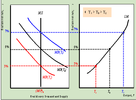
supply = real money demand). The graphical derivation of the LM curve is illustrated
below.

The left-hand side of the graph illustrates money market equilibrium for a given level
of Y. For example, when Y = Y0 the equilibrium real
interest rate is 5%. The right-hand-side of the graph gives the LM curve. The LM curve is
plotted with the real interest rate on the vertical axis and real income (GDP) on the
horizontal axis. Each point on the LM curve represents a money market equilibrium for a
particular real interest rate and income pair (r, Y). For example, the
money market equilibrium at (r = 5%, Y = Y0) is
given by the black (middle) dot on the LM curve.
At a higher level of income, Y1 > Y0, the money
demand curve shifts up and right and a new equilibrium occurs at r = 7%. This
equilibrium is represented by the blue (upper) dot on the LM curve. Similarly, at a lower
level of income Y2 < Y0 the money demand curve shifts
down and left and a new equilibrium occurs at r = 3%. This equilibrium is given
the by the red (lower) dot on the LM curve.
Factors that Shift the LM Curve
The above analysis shows that the LM curve is an upward sloping curve in the graph with
r on the vertical axis and Y on the horizontal axis. Every point on the LM curve
represents an intersection between the real money supply MS and real money demand
MD. The LM curve will shift whenever the variables we hold fixed, other than Y,
in the money-supply/money-demand diagram change. These variable are M/P and pe. In particular, if M/P increases holding
expected inflation fixed then r falls in the money market and so the LM curve
shifts down and right. Similarly, if expected inflation increases real money demand falls,
lowering the interest rate, and the LM curve shifts down and to the right.
The IS curve ("I" denotes investment and "S" denotes saving)
represents all combinations of income (Y) and the real interest rate (r)
such that the market for goods and services is in equilibrium. That is, every point on the
IS curve is an income/real interest rate pair (Y,r) such that the demand for
goods is equal to the supply of goods (where it is implicitly assumed that whatever is
demanded is supplied) or, equivalently, desired national saving is equal to desired
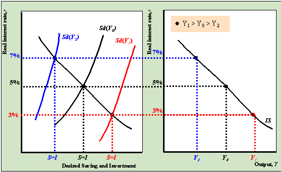
investment. The graphical derivation of the IS curve is given below.

Consider an initial equilibrium in the goods market where r = 5% and income is
equal to Y0. This equilibrium is illustrated in the graph on the right
with r on the vertical axis and Y on the horizontal axis as the big black dot (middle
dot). Now suppose Y increases to Y1 (say supply increases).
This increase in Y shifts the desired savings curve down and right lowering the
equilibrium real interest rate to 3%. The new equilibrium in the goods market with higher
income and a lower real interest rate is illustrated in the graph on the right as the big
blue dot (bottom dot). Similarly, if Y decreases from Y0 to Y2
then the savings curve shifts up and left and the equilibrium real interest rises. The new
equilibrium in the goods market with lower income and a higher real interest rate is
illustrated in the graph on the right as the big red dot (top dot). Notice that as income
increases (decreases) the real interest must fall (rise) in order to maintain equilibrium
in the goods market. This is the relationship that is represented in the downward sloping
IS curve.
Factors that Shift the IS Curve
Every point on the IS curve represents an intersection between desired national saving
and desired investment for some income/interest rate pair (Y,r). As such the IS
curve is derived holding the determinants of saving and investment, other than Y
and r, fixed. When these factors change the IS curve will shift. Since points on
the IS curve represent points where aggregate demand is equal to aggregate supply any
factor that increases the demand for goods and services will shift the IS curve up and to
the right and any factor that decreases the demand for goods and services will shift the
IS curve down and to the left. From the savings/investment diagram it follows that any
shift of the savings or investment curve that increases the real interest rate, holding Y
fixed, will shift up the IS curve.

