Last updated: January
16, 2000
Note: These notes are preliminary and incomplete
and they are not guaranteed to be free of errors. Please let me know if
you find typos or other errors.
Our discussion so far of the labor market and the production function represents the
supply-side of the economy independent of the overall level of aggregate demand. Changes
in factors that affect labor demand, ND, labor supply, NS and the
production function, F change the potential supply, Y*, of the economy
independent of demand. (Note: Here, variables with superscript "*" are
equilibrium values. In the textbook overbars "-" are used)
The demand-side of the economy focuses on the aggregate demand for goods and services
independent of potential supply. To simplify our analysis, we assume
- No foreign sector to the economy => NX = 0
Then aggregate demand for goods and services, using the expenditure approach, is
defined as:
Yd = Cd + Id
+ G0,
- Cd = demand for consumption goods
- Id = demand for investment goods
- G0 = exogenous (taken as given)
government spending on goods and services.
Modeling the aggregate demand for goods and services thus requires modeling the demand
for consumption goods and the demand for investment goods. However, since desired national
saving is defined as
Sd = Yd - Cd
- G0
we may also focus on modeling saving behavior instead of consumption behavior.
The aggregate supply of goods in the economy, AS, is
determined by the interaction of the production function with the labor market. That is, AS
= Y = full employment output.
Equilibrium in the market for goods and services occurs when the aggregate demand for
goods and services, defined as AD = Yd = Cd + Id + G0,
is equal to the aggregate supply of goods and services (real GDP), Y. In other
words, the goods market equilibrium condition
is
Yd = Y =Cd + Id
+ G0.
We may also express this goods market equilibrium in terms of desired national saving
and desired investment. By subtracting Cd +G0 from the left
and right hand sides of the equilibrium condition we get:
Y - Cd - G0 = Id.
Using the fact that, in equilibrium, desired national saving is defined as
Sd = Y - Cd - G0
we get the equivalent equilibrium condition:
Sd = Id.
Therefore, in our economy without a foreign sector we have
equilibrium in the market for goods and services if desired national saving is equal to
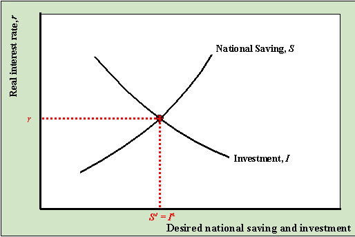
desired investment expenditure. We may represent this equilibrium condition in
a savings-investment diagram relating both desired national saving and investment as
functions of the real interest rate.

Equilibrium in the goods market can be expressed in two
equivalent ways: (1) desired national saving is equal to desired investment; AS =
AD. The graph at right shows that the real interest rate plays a key role in
determining goods market equilibrium.
In goods market equilibrium there are no forces acting on savers and investors to move
the real interest rate up or down. When the interest rate is such that desired saving is
not equal to desired investment then the goods market is not in equilibrium (it is in
disequilibrium) and there are market forces acting to move the economy back into
equilibrium.
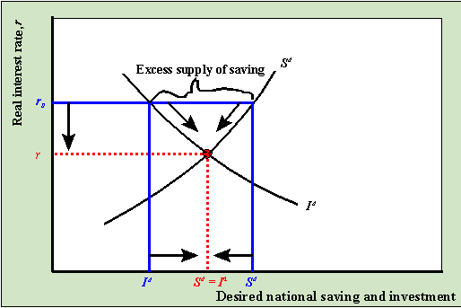
The diagram below illustrates a situation where the real interest rate is higher than
the equilibrium interest rate.

At r0 > r*, the return to saving is high
but the cost of investment is high so that desired saving is greater than desired
investment: there is an excess supply of saving. In this case, banks have more cash on
hand than they can loan out to firms. In order to create more loans banks must lower the
real interest rate. As r falls, we move down along the savings and investment
curves toward the equilibrium point r* where Sd = Id.
The term comparative statistics refers to the exercise of
shocking the market out of equilibrium and seeing what happens as the market adjusts to a
new equilibrium. Recall, the desired saving and investment curves are drawn for given
levels of certain variables like current income, Y, expected future income, Ye,
wealth, WL, government spending, G, and the expected future marginal
product of capital, MPKf. If any of these variable change - which
defines a shock to the market -then either the desired saving or investment curve will
shift and the goods market will go into disequilibrium. Competitive forces will then act
on the market to bring it back into equilibrium at the intersection of saving and
investment. The examples below illustrate the process.
Increase in current income (Y)
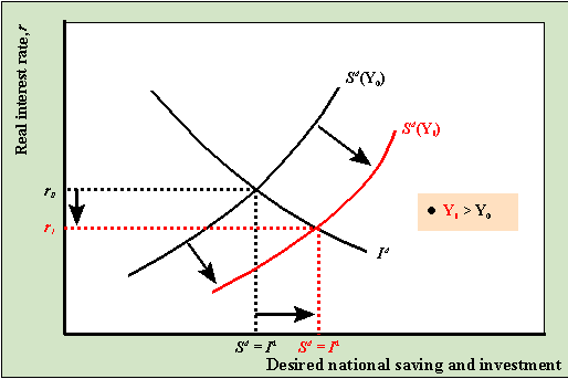
Suppose the goods market is initially in equilibrium with r* = 5% with current
income at Y0 as described in the diagram below. Now suppose that
current income (Y), which is equivalent to current output, increases from Y0
to Y1. This results in a rightward shift of the desired savings graph
as depicted below.

At r0 there is now an excess supply of saving
which puts downward pressure on the real interest rate as banks try to create more loans.
As r falls, we move along both the desired saving and investment graphs toward
the new equilibrium at r1. The end result of the increase in Y
is a lower real interest rate and a higher level of both saving and
investment.
Increase in the future marginal productivity of
capital (MPKf)
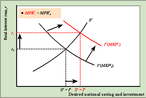
Now consider an increase in MPKf due to, say, an increase in
business confidence about future profits. This could occur, for example, if firms expect
that tax laws favoring business investment may be enacted in the near future. The increase
in MPKf leads to a rightward shift up in the desired investment graph
holding everything else in the model fixed as illustrated in the graph below.

At r0, desired investment is greater than
desired saving: there is an excess demand for saving. Accordingly, banks are able to
raise real interest rates due to the increased demand for loans. As r rises, we
move up along both the saving and investment graphs toward the new equilibrium at r1.

