Chapter 4

Two-Dimensional Problems

In two-dimensional problems,  displacement, strain, and stress components of interest, all lie in a plane. Taking that plane as the (x, y) plane, the variables of interest are functions of x and y only, and consists of:

Displacements: u, v

Strains:  e_x, e_y, g_xy

Stresses: s_x, s_y, t_xy

The other variables are not necessarily zero, but are determined in terms of the variables above.  Two types of two-dimensional problems seen earlier, Plane Stress and Plane Strain, are discussed in what follows for linearly elastic isotropic materials.

1. Plane Stress or Stretching of Plates

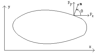The figure shows the middle plane of a plate , bounded by a curve of arbitrary shape, and typical tractions p_x and p_y at a point of the boundary.  The plate has a thickness t in the z direction, assumed to be small compared with the linear dimensions in the (x, y) plane.  The faces of the plate are stress- free.   A state of plane stress is one in which the loading is in the (x, y) plane, and is uniform in the z direction. Body force components F_x and F_y, functions of x and y only, may act, but F_z and p_z are zero.  Since the faces of the plate are stress free, it is reasonable to assume, subject to verification,  that s_z , t_zx, and t_zy  are zero throughout the plate, and thus also  g_zx, and g_zy.  From the stress-strain relations  e_z is not zero, because of Poisson's ration, but is determined in terms of e_x and e_y.

If one checks whether the six strain compatibility equations can be satisfied by the preceding assumptions, it turns out that some stress variation in the z direction, symmetric about the (x, y) plane,  is required.  However, for a thin plate, a small variation in that direction can be neglected, and the stresses may be considered constant along the thickness. 

An example of a state of plane stress was given in the chapter 'Analysis of Stress'.

The governing equations of plane stress were presented in Chapter 3, and are re-written below.

Equilibrium

s_x,_x + t_yx, _y + F_x = 0                   (1)

t_xy,_x + s_y,_y + F_y = 0

Strain-Displacement Relations - Compatibility

e_x = u,_x

e_y = v,_y                                       (2)                       

g_xy = u,_y + v,_x

Elimination of the displacements from the above equations yields the compatibility equation

e_x,_yy - g_xy,_xy  + e_y,_xx = 0             (3)

Stress-Strain Relations

Auxiliary Equation

e_z  is obtained from the condition s_z  = 0 as

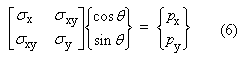
Boundary conditions

Typical boundary conditions are of stress type or of displacement type.  In a condition of stress type, a traction is prescribed on a boundary segment, and in a condition of displacement type, a displacement component is prescribed on a boundary segment.  For a well defined problem, two conditions are needed at each boundary point, one for each of  two directions at that point.  These can be the (x, y) directions, or the normal and tangential directions to the boundary.   Conditions prescribing tractions p_x and p_y  have the form

2. Plane Strain

A state of plane strain is one in which w = 0, and u and v are functions of x and y only.  A typical illustration is that of a long prismatic body of arbitrary cross sectional shape, whose length is in the z direction, and whose loading on the longitudinal boundary and in the domain does not vary with z, and has zero z-components.  A gravity dam would fit such a description.  Assume further that the end cross sections have smooth contact with planar support planes, so that w, t_zx, and t_zy are zero at the end cross-sections.  It is reasonable to assume, subject to verification,  that w, t_zx, and t_zy are zero throughout the plate, and thus also  g_zx, and g_zy.   Since w = 0, e_z = w,_z = 0.  From the stress-strain relations, s_z is not zero, because of Poisson's ration, but is determined in terms of s_x and s_y.   The preceding assumptions turn out to be fully consistent with the three-dimensional governing equations.

For a structure such as a gravity dam, actual boundary conditions at the end cross sections do not fit the plane strain assumptions.  However, by St-Venant's principle, a state of plane strain exits away from the ends.

The variables of the governing equations of plane strain are the same as those of plane stress.  The equilibrium and the strain-displacement relations are also the same.  The stress-strain relations are different, however.  In plane strain, e_z = 0, whereas in plane stress,  s_z = 0.  With e_z = 0, s_z is obtained form the stress-strain relations as

s_z = n(s_x + s_y)                        (1)

and the stress-strain relations take the form

Eqs. ( 2) and (2') may be obtained from those of plane stress by substituting in the latter

then renaming E' and n', E and n respectively.

3. Stress Method

The stress method determines the stresses first.  Its governing equations consist of the two equilibrium equations and of the compatibility equation expressed in terms of the stresses, which form a system of three differential equations in three unknown stresses.  The compatibility equation expressed in terms of the stresses by means of the stress-strain relations will be referred to as the stress compatibility equation.  The equation may be simplified with use of the equilibrium equations to yield, in the case of plane stress,

If the body force is zero, the equation reduces to

Functions that satisfy Eq. (2) are called harmonic. Since the elastic constants do not appear in the equation, it is applicable to both plane stress and plane strain. 

A general approach to the stress method known as the Airy stress function method is presented in Sec. 5.  In this section, inverse and semi-inverse approaches are used to solve simple but fundamental problems, some of which will be used both to justify and to shed some light on the limitations of engineering beam theory. 

Exercise 3.1

Obtain Eq. (1) by following the procedure described above.

Hint:  Group and adjust terms in the compatibility equation to obtain the terms in Eq. (1), then look in the remaining terms for expressions that are derivatives of the left hand sides of the equilibrium equations, and replace such expressions in terms of the body force components.

Solution by the Inverse and Semi-Inverse Approaches

The inverse approach consists in guessing the solution, based on insight or previous experience, and to check whether that guess satisfies the governing equations.  If some equation is violated, an improved guess may be tried.  The semi-inverse approach consists in making a partial guess, and trying to use the governing equations to solve for the remaining unknowns.

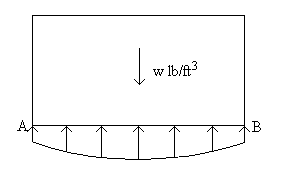
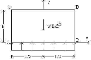
Example 1 - Wall Subjected to its Weight

A rectangular wall ABCD is in equilibrium under its weight w lb/ft³, and a uniform reaction along its bottom edge as shown.  Determine the stresses.

The body force components are

F_x = 0

F_y = -w

On the bottom edge, the uniform traction balances the weight of the plate, and is thus equal to

p_y = wh

A solution by an inverse method is attempted, based on the assumption that any vertical wall strip is in a uniaxial state of stress.  Thus at any level y, s_y balances the weight of what's above, as is the case at the bottom edge.  There is no apparent need for s_x and t_xy.  We thus assume, subject to verification, that

s_y = -w(h - y)

s_x = 0

t_xy = 0

We may verify that these stresses satisfy the boundary conditions and the equilibrium equations (Sec. 2, 1).  By inspection they also satisfy the compatibility equation (Sec. 4, 1).  The proposed solution is thus the exact solution for the stresses.  Determination of the displacements in the next section will shed additional light on this problem.

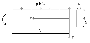
Example 2 - Thin Plate Acting as a Cantilever  Beam

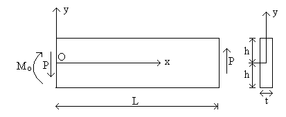The figure shows a rectangular plate of thickness t, subjected to the load P at x = L, and to balancing reactions P and M_o = PL at x = 0.  These are relaxed boundary conditions on the edges, x = 0 and x = L.  On the top and bottom edges the boundary conditions are s_y = 0 and t_yx = 0.

A semi- inverse method of solution is attempted based on the normal stresses of engineering beam theory.  Considering the plate as a beam spanning in the x direction, the bending moment is

M = P(L - x)

Letting I be the moment of inertia, we have

I = 2th³/3

and the normal stresses of engineering beam theory are

s_x = -My/I = -(P/I)(L - x)y

s_y = 0

It is verified that (s_x + s_y) satisfies the compatibility equation, Eq. (2).  There remains to determine t_xy, and to satisfy the equilibrium equations and the boundary conditions.

The equilibrium equations yield

s_x, _x + t_yx,_y =  (P/I)y + t_yx,_y = 0

t_xy,_x + s_y,_y =  t_xy,_x = 0

From the last equation, t_xy is independent of x, and from the preceding equation

 t_yx = ∫-(P/I)ydy = -(P/2I)y² + C

The boundary conditions,  t_yx = 0 at y = h and y = -h,  yield

C =  (P/2I)h²

To summarize, the proposed solution for the stresses is

s_x = -My/I = -(P/I)(L - x)y

t_yx =  (P/2I)(h² - y²)

s_y = 0

s_y  and t_yx satisfy the boundary conditions at the top and bottom edges, s_y = 0 and t_yx = 0.  There remains to check whether the relaxed boundary conditions at x = 0, and x = L are satisfied.  Since the stresses are the same as in engineering beam theory, it may be concluded that they do satisfy the relaxed boundary condition.

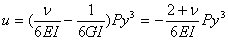
For a direct check of the relaxed boundary conditions, the stress resultants are evaluated in what follows at a general cross-section, which can be specialized to the ends x = 0, and x = L.  We have,

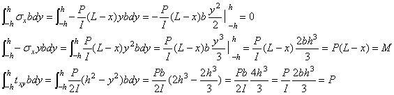
The first equation is the condition of zero axial force, the second equation verifies that the resultant moment over a cross section is the computed bending moment, and the last equation verifies that the resultant shear over a cross section is P. 

It is concluded that the stresses of engineering beam theory in this example form an exact elasticity solution, provided we adopt relaxed boundary conditions at the ends.  The displacements are obtained in a later example, where it will be seen that they differ in certain respects from those of engineering beam theory.

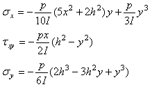
Example 3 - Thin Plate Acting as a Simple  Beam

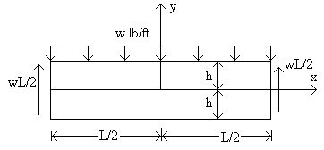The problem shown in the figure consists of a rectangular plate of thickness t, subjected on its upper edge to a uniform load w lb/ft, and at the left and right edges to balancing forces wL/2.  The boundary conditions are:

At y = h, s_y = -w/t, t_yx = 0 

At y = -h, s_y = 0, t_yx = 0

At x = L/2 and x = -L/2, we adopt the relaxed boundary conditions

There are also two conditions expressing that the resultant of the shear stress at each end acts upward and is equal to wL/2 .  These conditions will automatically be satisfied however, once the conditions M = 0 at the ends are satisfied, and the differential equilibrium equations are satisfied in the domain.

We will apply again a semi-inverse approach, using the stresses of engineering beam theory.  The shear force and bending moment are found as

V = wx

M = w(L²/8 - x²/2)

and the stresses according to beam theory are

(s_x)_b = -My/I = - (w/2I)(L²/4 - x²)y

(t_xy)_b = VQ/tI = (w/2I)x(h² - y²)

where subscript b refers to beam theory, and

I = 2th³/3

It is readily verified that the stresses above satisfy the first differential equation of equilibrium, and the boundary conditions at the ends of the plate.  The shear stress also satisfies its boundary conditions at the top and lower edges.  Since s_y is ignored in beam theory, we can obtain it by means of the second differential equilibrium equation, from which

s_y,_y = -t_xy,_x = -(w/2I)(h² - y²)

Integrating with respect to y yields

s_y = -(w/2I)(h²y - y³/3 + C)

where C is an arbitrary function of x, which will turn out to be a constant.  The condition,  s_y = 0 at y = -h, yields

C =  2h³/3

and

s_y = -(w/6I)(3h²y - y³ + 2h³)

At y = h,

s_y = -(w/6I)(3h³ - h³ + 2h³) = -2h³w/3I = -w/t

The s_y condition at the top edge is thus satisfied.

Except for the compatibility equation, which remains to be checked, all governing equations and boundary conditions are satisfied.  The compatibility equation yields

(s_x + s_y),_xx + (s_x + s_y),_yy = (w/I)(y + y) = 2wy/I

The stresses are thus not compatible, and need to be modified.

To satisfy the compatibility equation, let us superimpose on the preceding solution a stress (s_x)' such that

(s_x)',_xx + (s_x)',_yy = - 2wy/I

while continuing to satisfy the equilibrium equations and the relaxed boundary conditions.  We can do that by choosing  (s_x)' as a function of y only.  Thus

(s_x)',_yy = - 2wy/I

Integrating twice yields

(s_x)' = - (w/I)(y³/3 + Cy + D)

The relaxed boundary conditions at the ends,

which are satisfied by (s_x)_b must also be satisfied by (s_x)'.  It is found that the condition N = 0 yields D = 0, and the condition M = 0 yields C = -h²/5.

The final solution is thus

s_x = - (w/2I)(L²/4 - x²)y - (w/I)(y³/3 - h²y/5)

s_y = -(w/6I)(3h²y - y³ + 2h³)

t_xy = (w/2I)x(h² - y²)

Actual support conditions cannot provide the stress distributions at the ends that are required by the solution.  By St Venant's principle, however,  the solution becomes valid away from the ends, at distances comparable to the depth. The maximum correction to s_x is of the order (h²/L²) compared to the engineering theory value, and is thus negligible except for deep beams. 

Exercise 3.1

1. Find out whether the stress field

where

 is a valid solution of the plane stress problem shown in the figure.

2. How does this solution differ from that of engineering beam theory?

Exercise 3.2

Apply the semi-inverse method to determine the stresses in the plane stress problem shown.  Assume relaxed boundary conditions at x = 0, and x = L.

Hint:  Obtain the axial force N and bending moment M on a general section, as functions of x, and start with the normal stress s_x of engineering beam theory.

Exercise 3.3

The problem of Exercise 3.1 may be formulated as the superposition of the problems of Examples 2 and 3.  Obtain the solution on that basis.  Note that the solutions of examples 2 and 3 need to be represented in the same axes of reference before superposition can be made.

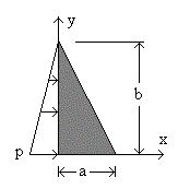
Exercise 3.4

Use a semi-inverse method to determine the stresses in the plane stress problem shown.  The pressure p is defined per unit area.  Assume relaxed boundary conditions at the bottom boundary.

Hint: Assume s_y to be linear in x, so it is obtainable by a beam flexure formula on a section y = constant.

4.  Determining the Displacements in the Stress Method

Having determined the stresses, the strains are determined using the stress-strain relations, and the displacements are obtained by integration of the strain-displacement relations.  The integration is possible, because one of the governing equations insures that the strains are compatible.  Since there are no support conditions in the stress method, the solution for the displacements contains an arbitrary rigid body displacement.   Recall, however,  that the linear theory is limited to small rotations.  An example of determining displacements from strains may be seen in Chapter 2, Sec. 7, Example 2.  The displacements of two preceding examples are determined in what follows.

Example 1.  (Sec. 3, Example 1)

The displacements for Example 1, Sec. 3,  are determined in what follows.  Substituting the solution for the stresses into the strain-displacement-stress  relations yields

u,_x = -ns_y/E = nw(h-y)/E

v,_y = s_y/E = -w(h-y)/E

u,_y + v,_x = t_xy/G = 0

Integrating the first two equations yields

u = nwx(h-y)/E + f(y)

v = -w(hy-y²/2)/E + g(x)

Substituting into the third equation, and putting all terms on one side, yields

f '(y) + g '(x) - nwx/E  = 0

The left hand side of this equation is a sum of a function of y and a function of x, which must be zero for all x and y.  For this to be possible the two functions must be constant and add up to zero. Thus

g '(x) - nwx/E   = c

f '(y)  = -c

then

g(x) = nwx²/2E + cx +  b

f(y) = - cy + a

and

u = nwx(h-y)/E - cy + a

v = -w(hy-y²/2)/E + nwx²/2E + cx +  b

where a, b, and c are integration constants representing a rigid body displacement. a and b are translations in the x and y directions, respectively, and c is a rotation about the origin.

Any support conditions against rigid body displacements, without over-constraining the body, can be prescribed without changing the solution for the stresses.  We can for example set the displacements of the mid-point of AB to zero, and set the rotation of the horizontal fiber at that point to zero.

Thus, at (x = 0, y = 0), 

u = a = 0

v = b = 0

v,_x =  c = 0

The displacements reduce to

u = nwx(h - y)/E 

v = w(y² - 2hy + nx²)/2E

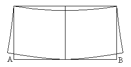
It is seen that if n is not zero, material lines, y = constant, have a vertical displacement that varies as x², and a horizontal displacement linear in x.  Such lines deform into parabolas. Vertical lines also deform as parabolas.  The deformed horizontal and vertical lines remain orthogonal, since the shear strain is zero in the domain.  The deformed shape of the wall is shown in the figure, which shows that if the wall is supported along AB, a uniform reaction is impossible since it implies lifting of the wall edge, and this in turn is inconsistent with the support exerting a reaction.  The proper formulation of support conditions along edge AB is to prescribe v = 0 on that edge instead of a uniform reaction.  The solution of the problem becomes more complicated, and may need to be found by numerical methods.  Qualitatively, in order to maintain contact with a rigid support along AB,  we need to superimpose on the previous problem a new one in which the traction along AB tends to straighten the edge while having a zero resultant.  The resulting reaction would decrease near A and B, and would increase near the center, and would look as shown in the figure. 

Example 2. (Sec. 3, Example 2.)

To determine the displacements for the present example, we substitute the solution for the stresses of Sec. 3, Example 2, into the strain-displacement-stress  relations.  This yields

u,_x = s_x/E = -(P/EI)(L - x)y

v,_y = -ns_x/E = (nP/EI)(L - x)y

u,_y + v,_x = t_xy/G= (P/2GI)(h² - y²)

Integrating the first two equations yields

u =  -(P/EI)(Lx - x²/2)y + f(y)

v = (nP/EI)(L - x)y²/2 + g(x)

Substituting into the third equation, and putting all terms on one side, yields

-(P/EI)(Lx - x²/2) + f '(y) - (nP/EI)y²/2 + g '(x) - (P/2GI)(h² - y²) = 0

The left hand side of this equation is a sum of an expression function of x and another expression function of y, which must be zero for all x and y.  For this to be possible the expressions must be constant and add up to zero. Thus

g '(x) -(P/EI)(Lx - x²/2)  = c

f '(y) - (nP/EI)y²/2 - (P/2GI)(h² - y²) = -c

then

g(x) = (P/EI)(Lx²/2 - x³/6) + cx +  b

f(y) = (nP/EI)y³/6 + (P/2GI)(h²y - y³/3)  -cy + a

and

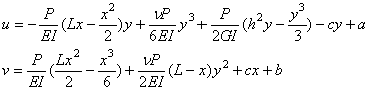
where a, b, and c are integration constants representing a rigid body displacement. As in the previous case, a and b are translations in the x and y directions, respectively, and c is a rotation about the origin.

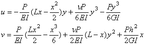
Any support conditions against rigid body displacements, without over-constraining the body, can be prescribed without changing the solution for the stresses.   For the purpose of comparison with a cantilever,  let the origin point be fixed, and the rotation of the vertical material fiber at that point, (u,_y), be zero. The conditions u = 0, and v = 0 at point (x = 0, y = 0) yield a = 0, and b = 0.  The condition  u,_y = 0 at the same point yields

c = Ph^2/2GI

Thus, finally

Comparison with a Cantilever Beam

The solution of the preceding problem offers some points for comparison with the beam-theory solution of a cantilever fixed at the edge x = 0.

a) The stresses are the same in both solutions, but the displacements differ.  For example, at  x = L, we have

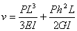
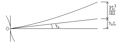The first term coincides with the deflection of beam theory.  The second term is associated with shear deformation, as the presence of the shear modulus indicates. The shear strain at the origin is 

g_o = Ph²/2GI

and the term Ph²x/2GI  in the expression of v, is equal to g_ox, which is a rotation about the origin by the angle g_o.  The figure shows the deflection of the centerline and the part due to shear.  It also shows the distorted shape of the cross section at x = 0.

b) The edge x = 0 is fixed in the beam-theory model of a cantilever, whereas in the present solution the edge has a non zero strain e_y due to Poisson's ratio, and it distorts out of the plane of the cross section because of shear deformation, as shown in the figure.  At x = 0,

c) The present solution is valid if the stresses acting on the left and right edges are in fact distributed as found.  If not, by St-Venant's principle, the stresses are valid away from the ends.  Beam theory by contrast ignores such details.  For a long plate, a different stress distribution near the ends causes only a local change in strains, and thus should not significantly affect the maximum deflection.  The deflection due to shear is an improvement over the usual engineering beam theory, which ignores such a term. However, the distortion of the left edge does not satisfy the fixity of an actual cantilever.  The deflection due to shear may thus be expected to be larger than would occur if the edge were fixed, since such fixity would further restrain the deformation.  A shear deflection term that more accurately describes an actual cantilever may be based on an energy method, and is found to be 5/6 of the term found by the elasticity solution for a rectangular cross section.

Exercise 4.1

Determine the displacements in the problem of  Sec. 3, Example 3.  Keep the symbol G for the shear modulus so that the terms associated with shear deformation can be traced. Assume support conditions that try to represent a simply supported beam.  Compare the deflection at mid span of the centroidal line with that of engineering beam theory.

Exercise 4.2

Determine the displacements in the problem of Sec. 3, Exercise 3.1.  Keep the symbol G for the shear modulus so that the terms associated with shear deformation can be traced. Assume support conditions that try to represent a cantilever fixed at x = L,  by requiring the vertical material fiber to have a zero rotation.  Compare the deflection at (x = 0, y = 0) with that of engineering beam theory.

5. Solution by Airy's Stress Function

Assuming the body force is zero, the equilibrium equations are solved by the expressions

s_x = F,_yy

s_y = F,_xx                             (1)

t_xy = -F,_xy

where F is an arbitrary differentiable function, called Airy's stress function. This may be verified simply by substituting into the equilibrium equations, and noting that in mixed partial derivatives the order of derivations is commutable. The compatibility equation yields the differential equation governing F.  We have, in the case of zero body force,

and the compatibility equation takes the form

This is known as the biharmonic equation, and functions satisfying it as biharmonic functions.  The equation occurs frequently in mathematical physics, and has various forms of analytical solutions applicable to two-dimensional elasticity problems, among which solutions in the forms of polynomials and Fourier series.  See for example 'Theory of Elasticity' by Timoshenko and Goodier.

Example 1

Solve the problem shown by Airy's stress function.

Using beam behavior as a guide, the bending moment is equal to p(L-x)h, which is linear in x.  let us try a stress function that yields s_x as linear in x and y, and t_xy as independent of x and parabolic in y.   Since s_x = F,_yy, F should contain terms of the form y³(ax + c) + dy², and since  t_xy = -F,_xy,  F should contain terms of the form x(c'y³ + ey² + fy).   Let us try then

F = y³(ax + c) + dy² + x(ey² + fy)                 

First, check whether F satisfies Eq. (3).  It is seen that all fourth derivatives that appear in Eq. (3) are zero, and Eq. (3) is thus satisfied.  The stresses given by F are

s_x = F,_yy = 6y(ax + c) + 2d + 2ex         (E1)

s_y = F,_xx  = 0                                        (E2)

t_xy = -F,_xy = -3ay² - 2ey - f                  (E3)

What remains is to satisfy the boundary conditions.  At the top and bottom edges, the condition s_y = 0 is satisfied.  The other boundary conditions consist of:

a)  Top and bottom edges:  t_xy = p/b at y = h, and t_xy = 0 at y = -h.  Thus

-3ah² - 2eh - f  = p/b              (E4)

-3ah² + 2eh - f = 0                 (E5)

b)  At x = L, using relaxed boundary conditions,

or,

ah² + f = 0                     (E6)

d + eL = 0                     (E7)

c + aL = 0                     (E8)

Eqs. (E4) to (E8) form 5 equations to determine the 5 constants a, c, d, e, and f.

Subtracting and adding Eqs. (E4 and E5) yields

e = -p/4bh                                             (E9)

-3ah² - f  = p/2b                                    (E10)

From Eqs. (E6) and (E10)

a = -p/4bh²

f = p/4b

and from Eqs. (E7) and (E8)

d = pL/4bh

c = pL/4bh²

Finally, substituting into Eqs. (E1) and (E3)

s_x = 6y(ax + c) + 2d + 2ex  = (3p/2bh²)y(L - x) + (p/2bh)(L - x)

t_xy  = -3ay² - 2ey - f  =  (p/4bh²)(3y² + 2hy - h²)

Exercise 5.1

a) Show that any polynomial in (x, y) of combined degree less than 4 is a valid Airy stress function.

b) Show that terms x³y and xy³ are valid in any Airy stress function.

c) Given the 4th order homogeneous polynomial ax⁴ + bx²y² + cy⁴, what relationship must exist between the coefficients for the polynomial to be a valid Airy stress function?

Exercise 5.2

In Example 1, let the load on the top edge be perpendicular to the edge, and vary linearly from 0 at x = 0 to p_o at x = L.  Using beam behavior as a guide, what polynomial terms would you include in an Airy stress function in an attempt to solve the problem?

6. Thermal Problems

The stress strain relations considered so far are assumed to hold at a reference temperature at which the undeformed geometry is defined.  If a temperature change, T = T(x, y, z), takes place, the stress-strain relations need to be modified to take into account the effect of temperature.  It will be assumed that the temperature change is not of such a magnitude as to affect E and n, and that the material has a constant coefficient of thermal expansion a.  A small, unrestrained, and isotropic material element, subjected to a temperature increase T, undergoes a free thermal expansion, which consists of an extensional strain

e_T = aT                        (1)

in all directions, and no shear strain  for any pair of orthogonal directions.  e_T is called the free thermal strain.  A free thermal deformation is by definition one that is stress-free.  If the material element is also subjected to stresses, elastic strains take place in addition to the thermal deformation.  Typical stress-strain-temperature relations have then the form

e_x  =  aT   +  (s_x -  ns_y -  ns_z)/E            (2)

g_xy = t_xy/G

with similar relations for the remaining strains and stresses.

Plane Stress

For plane stress,  s_z = 0, and T = T(x, y).  The stress-strain-temperature relations take the form

e_x  =  aT   +  (s_x -  ns_y)/E

e_y  =  aT   +  (s_y -  ns_x)/E                     (3)

g_xy = t_xy/G

The inverse relations may be obtained by substituting (e_x - aT) for e_x, and (e_y - aT) for e_y in Eqs. (Sec. 1, 4').  This yields

s_x  =  [E /(1-n²)](e_x  +  ne_y) -  EaT /(1-n)

s_y  = [E /(1-n²)](e_y  +  ne_x) -  EaT /(1-n)             (3')

t_xy = Gg_xy

The state of zero strain, referred to as the fixed state, plays an important role in understanding and analyzing thermal effects.  If  e_x, e_y, and g_xy are constrained to be zero, stresses are set up as given by Eqs. (3').   Using subscript F to refer to the fixed state, Eqs. (3) yield

(s_x)_F = (s_y)_F  =  - EaT/(1 - n)                   (4)

(t_xy)_F = 0

If a free thermal deformation is first allowed, the stresses required to cause elastic strains equal and opposite to the free thermal strains, thus resulting in the fixed state, are those given by Eqs. (4). 

Another consideration for understanding thermal effects is to describe under what conditions a free thermal deformation is possible in a finite body. 

To answer that question consider an unrestrained body subjected only to a temperature change T = T(x, y).  If a free thermal deformation is possible, the stresses would be zero, and the strains would be e_x  =  aT , e_y  =  aT , and g_xy = 0.  These strains are geometrically possible if they satisfy the compatibility equation, Eq. (Sec.1, 3), which yields, after dividing through by a,

T,_xx + T,_yy = 0                                        (5)

Thus T(x, y) must be a harmonic function.  If  T satisfies Eq. (5), the displacements of the unrestrained body, obtained from the free thermal strains, contain an arbitrary rigid body displacement.  Thus, if the body is supported against such displacements, without additional restraints, a free thermal deformation remains possible. 

If either T(x, y) is not harmonic or the body is over-supported, a free thermal deformation cannot take place.  Stresses are then set up that cause elastic strains, which when superimposed on the free thermal strains, result in compatible strains.  Note that if T(x, y) is not harmonic, neither the elastic strains nor the free thermal strains are by themselves geometrically possible, but only their sum is.

In three-dimensional elasticity, exact conditions for a free thermal deformation require that the six compatibility equations be satisfied, and this leads to the requirement that T must be linear in (x, y, z).  The reason Plane Stress does not require such a stringent condition is that, from the point of view of three-dimensional elasticity, Plane Stress is an approximation that satisfies geometric compatibility only in the (x, y) plane.  The error involved in violating other compatibility equations may be shown to be negligible for thin plates. 

In Engineering Theories, thermal problems need to be formulated within the context of such theories, as will be seen for beams.

Exercise 6.1

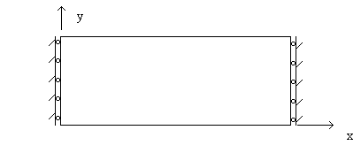
The rectangular plate shown has properties E, n, and a.  It is subjected to a constant temperature increase T, and is restrained in the x direction at the edges perpendicular to the x axis. Obtain the stresses and the displacements.

Hint:  Try a semi inverse approach.

Exercise 6.2

Let the sides of the plate of Exercise 6.1 be a in the x direction, and b in the y direction, and let the temperature increase in the plate be linear in y, with values T = T₁ at y = 0, and T = T₂ at y = b.

a) Obtain a complete solution for stresses and displacements.

b) Obtain the normal force N and moment M_C at the restrained edges, where M_C is the moment at the mid-point C of an edge.

.

7. Formulation in Polar Coordinates