Tom Trogdon

Let $H > 0$ be a positive-definite $N \times N$ matrix, and let $x_0$ be an $N$-dimensional random vector. The power method to compute the largest eigenvalue of $H$ is given by the iteration, for $j = 1,2,\ldots$ $$y_j = x_{j-1}/\|x_{j-1}\|_2,$$ $$x_j = Hy_j,$$ $$\mu_j = x_j^* y_j.$$ Then $\mu_j \to \lambda_{\max}$, the largest eigenvalue of $H$ as $j \to \infty$. With P. Deift, we considered the case where $H = XX^*/M$ is a sample covariance matrix. Here $X \in \mathbb C^{N \times M}$ has independent entries with mean zero and variance one (and some technical tail assumptions, $X$ could be real or complex as well). Define the (random) iteration count $$ T(H,x_0,\epsilon) = \min\{ j: |\mu_j - \mu_{j-1} | < \epsilon^2 \}. $$ The algorithm is terminated when the difference of two successive iterations is small. We proved the following universal, average-case theorem for $T$:

Theorem: Let $\epsilon \ll N^{-5/3 - \sigma}, \sigma > 0$ and $M \sim N/d$, $0 < d < 1$. Then there exists a distribution function $F_\beta^{\mathrm{gap}}(t)$ and a constant $c$ depending only on $d$ such that $$ \lim_{N \to \infty} \mathbb P \left( \frac{ T(H,x_0,\epsilon)}{c N^{2/3} (\log \epsilon^{-1} - \frac{2}{3} \log N)} \leq t \right) = F_\beta^{\mathrm{gap}}(t), \quad t \geq 0.$$ Furthermore, the distribution function $F_\beta^{\mathrm{gap}}(t)$ can be identified as the limiting distribution, after rescaling, of the inverse of the top gap in the real ($\beta =1$) and complex ($\beta = 2$) cases. This theorem gives both universality for and the average-case behavior of the power method. Similar results hold for the inverse power method, the QR algorithm and the Toda algorithm.

Consider the solution of the following initial value problem (IVP): $$i q_t = \omega(-i \partial_x) q, ~~ (x,t) \in \mathbb R \times (0,T),$$ $$q(x,0) = q_o(x), ~~~ \omega(k) = \omega_n k^n + \mathcal O(k^{n-1}) ~~ \text{is a polynomial.}$$ Provided the imaginary part of $\omega(k), k \in \mathbb R$ is bounded above this IVP is well-posed for $q_o \in L^2(\mathbb R)$. Now, consider the case where $q_o$ is piecewise continuous with a (piecewise) $L^2(\mathbb R)$ derivative then I (with G. Biondini) found a short-time expansion of the solution as $t \downarrow 0$. Furthermore, the expansion is computable numerically with high accuracy.

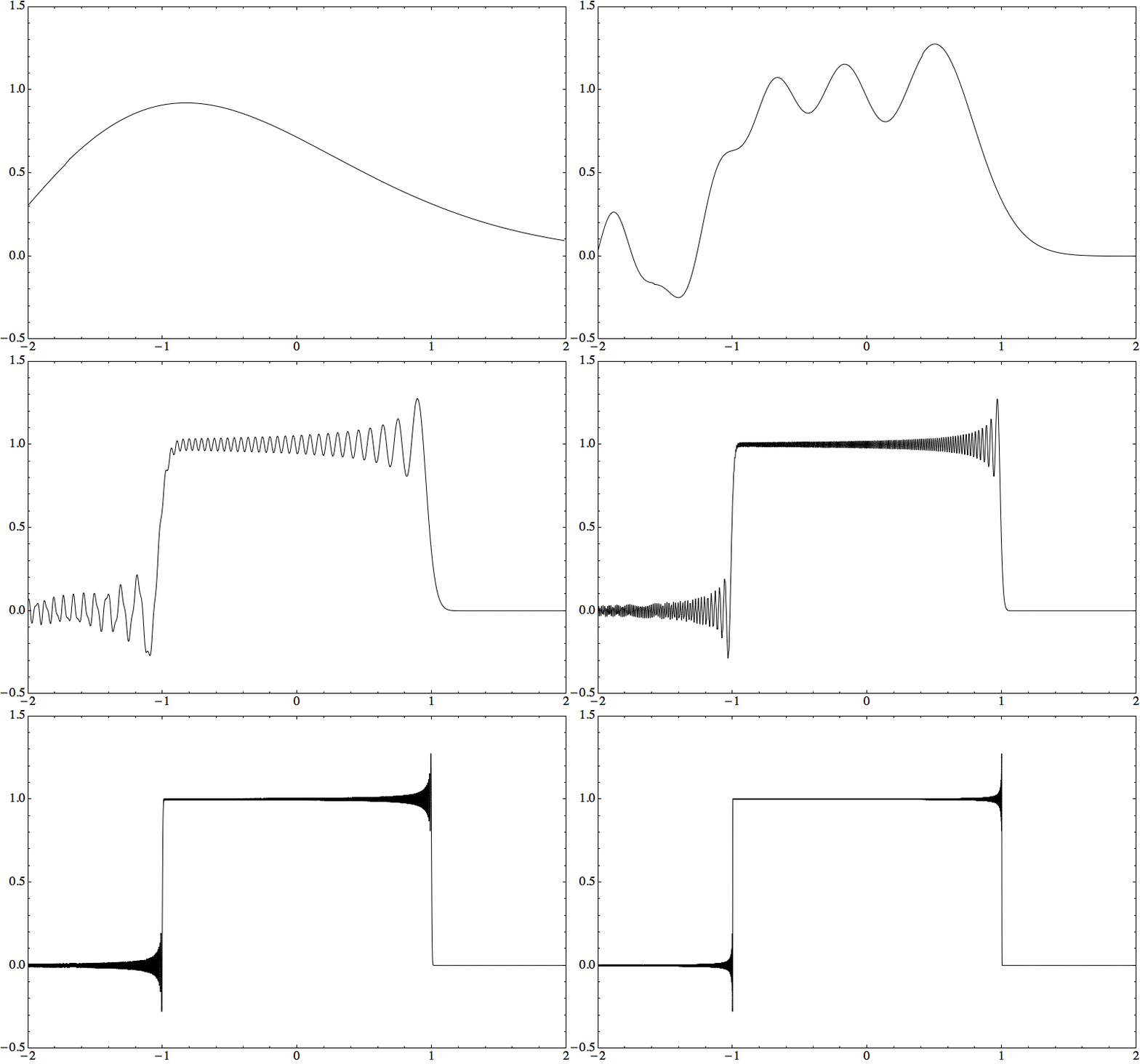
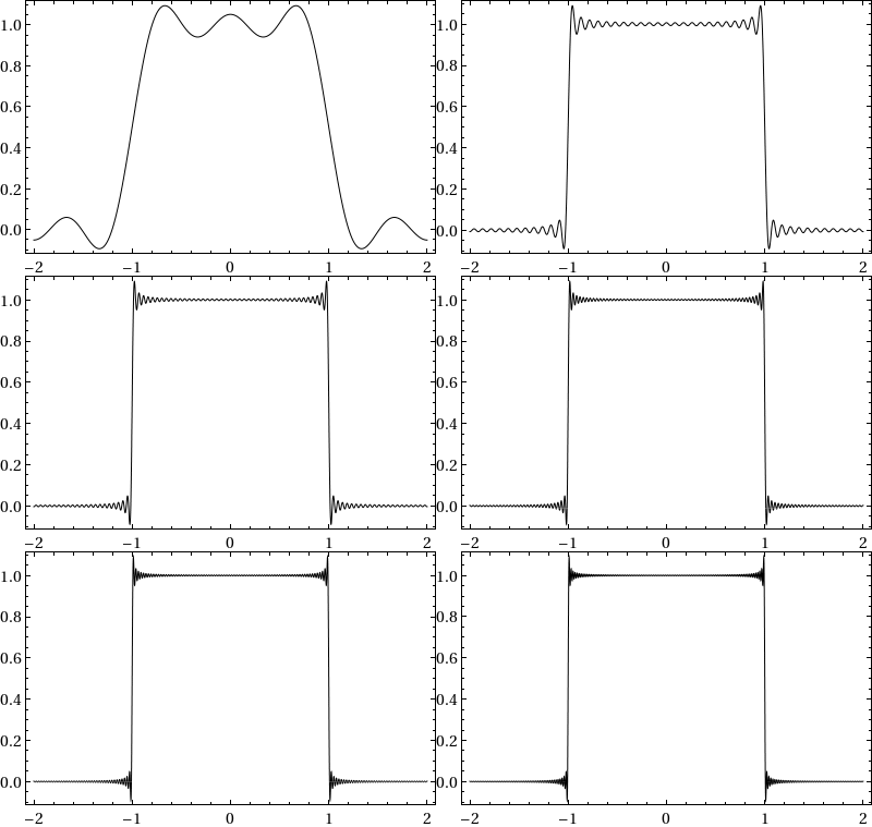
To illustrate the results let $$ q_o(x) = s(x)= \begin{cases} 1, & \mbox{if } |x| \leq 1,\\ 0, & \mbox{if } |x| > 1. \end{cases}$$ The behavior of the solution as $t \downarrow 0$ is seen in the animation below to mirror that of Gibbs phenomenon in Fourier series approximations.

Left/Top: $q(x,t)$ with $q_o(x) = s(x)$, $\omega(k) = -k^3$ as $t \downarrow 0$. Right/Bottom: A Fourier series partial sum approximation $S_n[s](x)$ of $s(x)$ as $n \rightarrow \infty$.

The effective computation of the inverse scattering transform, orthogonal polynomials with exponential weights, the Painlevé transcendents and other nonlinear special functions is accomplished by combining the Deift and Zhou method of nonlinear steepest descent with a method for the numerical solution of Riemann-Hilbert problems. Under mild assumptions on the numerical method, this combination produces an approximation that is uniformly and spectrally convergent over large parameter ranges. Below we plot a solution of the Korteweg-de Vries (KdV) equation while simultaneously displaying the contours of the Riemann--Hilbert problem that is being solved to compute the value of the solution q at each point.

Riemann-Hilbert methods are also used to derive representations of the finite-genus solutions of the KdV equation. This presents an alternative to the now-classical theta function approach. The Riemann-Hilbert problem is derived by representing scalar-valued analytic functions on a hyperelliptic Riemann surface by vector-valued functions on a cut version of the complex plane. These vector-valued functions satisfy a Riemann--Hilbert problem which can be solved numerically. An animation of a genus two solution of the KdV equation is found here:

A genus two solution of the KdV equation

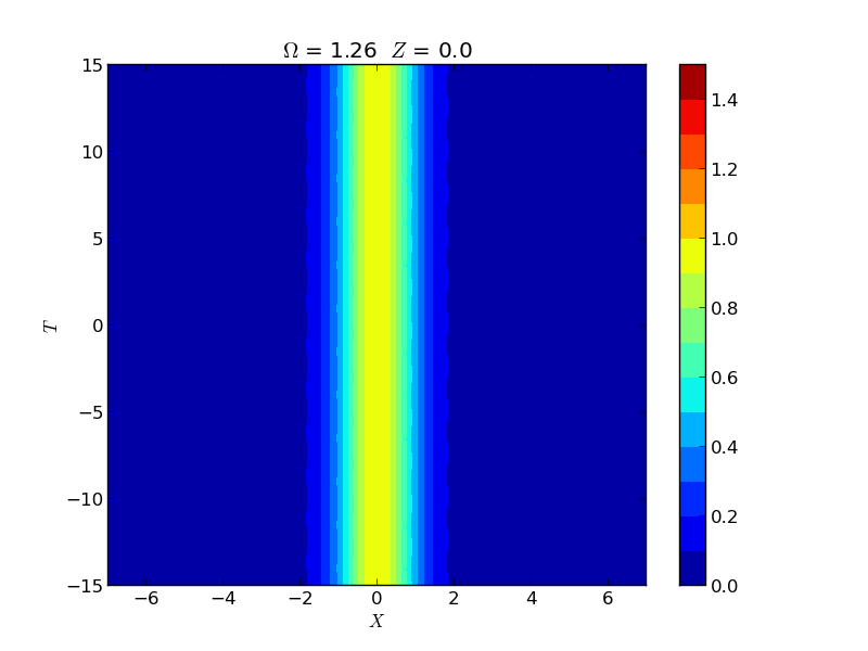
Instabilities of spatial solitons in a (2+1)-dimensional nonlinear Schrödinger equation have been well-studied since the work of Zakharov and Rubenchik in 1979. Through accurate computations using Hill's method we closely examine the growth rate of instabilities. Hill's method allows us to not only capture the maximal growth rate in the so-called snake and oscillatory snake regions but also the growth rate for the sub-dominant oscillatory neck instability. These rates are experimentally demonstrated by the group of M. Haelterman using a 2D waveguide array. See below for the computations of these instabilities. We animate the evolution of the equilibrium solution plus the first-order correction obtained using Hill's method.

Evolution of the neck instability

Evolution of the oscillatory snake instability