Fitting a model

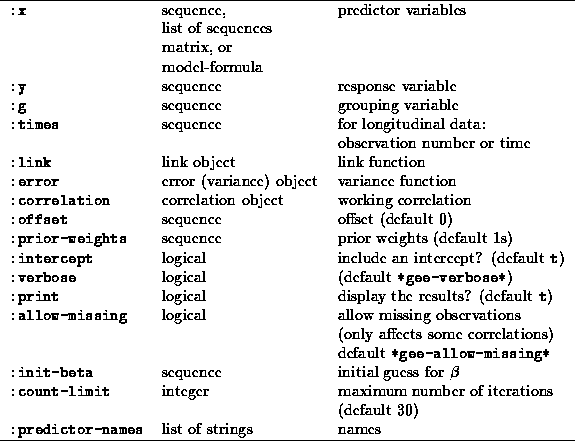
There is a wrapper function gee-model which takes the following arguments

You must specify the first three arguments and at least one of :link and :error. If only one of :link and :error is present then the other is set to a default value given in Table 1. If :correlation is not specified then the value of the global variable *gee-default-correlation* (typically the independence working model) is used. If :verbose is true the package will print a message indicating that these default choices have been used.

Note that for binomial data it is necessary to use the observed proportion not the observed count as the response and then to specify the denominators using :prior-weights. Correlated binomial data (other than binary) are comparatively rare; the individual binary observations are usually available.

The independence and exchangeable correlation structures ignore the observation :times argument, for other structures it is always required (in contrast to other packages). This is a feature, not a bug. The GEE functions written for other general-purpose packages mostly assume the data are sorted so that each group is contiguous and in the right order. In my experience data do not naturally occur that way. If the times column is in the data set it is easy to use it, if it isn't it is hard to be confident that the ordering is correct (and virtually impossible with missing observations). The performance implications of this and some theoretical considerations with missing data are discussed later.

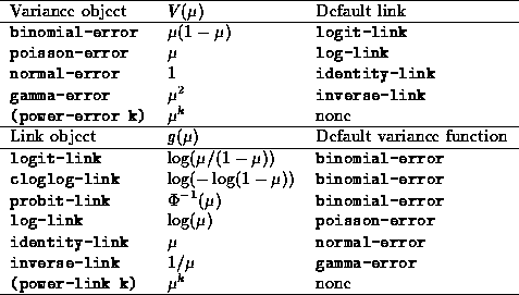
The default pairs of variance and link functions are given in Table 1.

  
Table 1: Default link and variance functions

These defaults are stored in the variables default-link and default-error. Most of these are well-known standards for generalised linear models. The use of power link and variance functions in modelling data with non-Normal, skew error distribution was discussed by Nelder (1994). The link functions are taken from the glim-proto system but have had extra methods :valideta and :validmu added to allow domain checking. Any link-variance combination is allowed and the program will usually find a solution even for badly-fitting combinations.

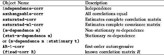
The available working correlation structures are described in Table 2. The parameter :allow-missing controls the assumptions made when the observation times are not the same for every group. Under the exchangeable and independence models it has no effect; under the other models unbalanced data are not allowed when :allow-missing is nil. When :allow-missing is t unbalanced data are allowed and the correlation parameters are estimated from the available data.

  
Table 2: Working correlation structures.

There is no need for the observation times to be consecutive integers. In fact they need not be integers at all, or even numbers. The requirements are that equalp is a valid test for equality and that rank will rank them. This means in practice that they must be all numbers or all strings and that if they are string the correct order is alphabetic. Group identifiers may also be either strings or numbers.

The following example uses the data set described in section 2 to fit the stationary 3-dependence model discussed there. All the example code can be found in the file example.lsp. The files geetest.lsp and geetestout give further examples to test the function and compare its results to the S-PLUS gee() function by Carey & Macdermott.

>(load "gee.1.0.lsp")
; loading "gee.1.0.lsp"
; loading "/usr/local/lib/xlispstat/Autoload/glim.fsl"
; loading "modelformula.lsp"
T
>(load "karim.lsp")
; loading "karim.lsp"
T
>(def example1 (gee-model :y num-visits :x (list sex smoke age time2 
time3 time4) :g id :error poisson-error :correlation (stat-m-dependence 3)
 :times times :predictor-names (list "sex" "smoker" "mother's age"
 "2nd vs 1st" "3rd vs 1st" "4th vs 1st")))
No link specified - canonical link used
Iteration 1: quasideviance = 517.114
Iteration 2: quasideviance = 478.439
Iteration 3: quasideviance = 475.966
Iteration 4: quasideviance = 476.062
Iteration 5: quasideviance = 476.087
Iteration 6: quasideviance = 476.088
Iteration 7: quasideviance = 476.088

GEE Estimates:

                         Coefficient     Std Error           Naive Std Error
Constant                  0.240922      (0.364061)          (0.360940)
sex                      -0.205502      (0.203637)          (0.220660)
smoker                    0.176987      (0.236101)          (0.240601)
mother's age               3.157128E-3  (6.490476E-3)       (6.210925E-3)
2nd vs 1st               -0.435318      (0.195649)          (0.190492)
3rd vs 1st               -0.307485      (0.202848)          (0.185973)
4th vs 1st                -1.12847      (0.221787)          (0.227792)

Scale Estimate:            1.83565    
Independence model deviance:   476.088    
Number of cases:               292
Link:                    #<Glim Link Object: LOG-LINK>
Variance function:       Poisson error
Stationary  3 - dependence Working Model: 
 correlation matrix =
#2a(
    (  1.0      0.21      0.19      0.34    )
    ( 0.21       1.0      0.21      0.19    )
    ( 0.19      0.21       1.0      0.21    )
    ( 0.34      0.19      0.21       1.0    )
   )
EXAMPLE1

Adding :verbose nil to the arguments will suppress everything before the line GEE Estimates. Adding :print nil will suppress everything from that point on.

The function returns a gee-proto object (in this case it is stored in the variable example1) that responds to a lot of messages, including many of the messages implemented for generalised linear models. Some description of most of the methods is available using the :help method (eg (send example1 :help :scale) describes the :scale method. To find all the methods which have help omit the topic specifier: (send example1 :help).

There is also a method for producing confidence intervals for the coefficients, transformed to any appropriate scale. The message :conf-interval gives the estimates and a 95% confidence interval. There are three optional keyword arguments: :coverage specifies the desired coverage, :names is nil to prevent predictor names being returned and :transform specifies a function to apply to the confidence interval. As an example we produce produce 90% confidence intervals for the hazard (incidence density) ratio in the example model above

>(print-matrix (send example1 :conf-interval :transform #'exp :coverage 0.9))
#2a(
    (Intercept         1.27242       0.699139        2.31579    )
    (sex              0.814238       0.582483        1.13820    )
    (smoker            1.19362       0.809480        1.76004    )
    (mother's age      1.00316       0.992509        1.01393    )
    (2nd vs 1st       0.647059       0.469010       0.892700    )
    (3rd vs 1st       0.735294       0.526692        1.02652    )
    (4th vs 1st       0.323529       0.224636       0.465959    )
   )
NIL