How the model works
Overview
LiveOcean works a lot like the weather forecast models that we all rely on every day. It takes in information about the state of the ocean, atmosphere and rivers on a given day, and then uses the laws of physics (and a large computer) to predict how the state of the ocean in our region will change over the next few days. The things that the model predicts are currents, salinity, temperature, chemical concentrations of nitrate, oxygen, carbon, and biological fields like phytoplankton, zooplankton, and organic particles. It does this in three dimensions, and allowing continuous variation over the full 72 hour forecast it makes every day.
The grid


The model grid is shown here for the full domain and for a close up of Puget Sound. The model horizontal resolution is 500 m in the Salish Sea and near the Washington coast, growing to 3 km at the offshore boundaries. It is designed to seamlessly simulate the interactions of the coastal ocean, the coastal estuaries like the Columbia River, Willapa Bay and Grays Harbor, as well as the whole Salish Sea (Puget Sound, the Strait of Georgia, and the Strait of Juan de Fuca). It has 279 rivers (cyan dots) and wastewater treatment plants (magenta dots). Vertically the model grid has 30 layers, distributed between the sea surface and the sea floor, with closer grid spacing near the surface and bottom to better resolve these important regions.
The model framework
The model framework we use is called the Regional Ocean Modeling System (ROMS) which is a large, flexible computer code that is used by coastal and estuarine oceanographers around the world to simulate different regions. It is known to have excellent numerical properties, such as low numerical diffusion, many choices for turbulence parameterization and open boundary conditions, built-in biogeochemical models, and a large, active user community. We have been using ROMS for realistic simulations in the region for research projects for the past decade and have found it to be a robust tool.
Bathymetry
To format the model for our region we first need to define the region and the grid size. The grid has to have fine enough resolution to resolve important physical processes like headland eddies and internal waves, but it also has to run fast enough to allow extensive testing. The current configuration is optimized based on our experience with previous projects. The bathymetry, or bottom depth, comes from a variety of sources, including a compilation of Puget Sound data made at UW.
Model forcing
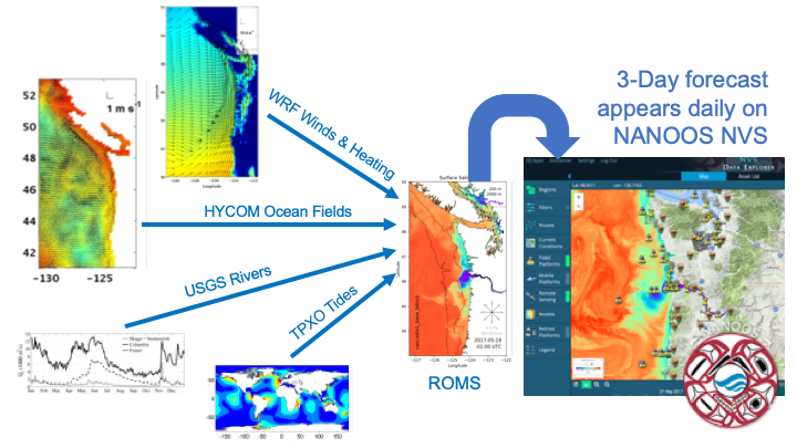
The environmental information we use to force the model comes from the outer boundaries. At the sea surface we force the model with winds, heating by sunshine, and other exchanges of heat with the atmosphere like evaporation. The atmospheric fields come from the regional weather forecast model run by Dr. Cliff Mass' group at UW. Weather models tend to make fairly good forecasts (at least for a few days) because they are initialized each day using observations from the real world. The same is true of the forcing of the ocean state we use at the open boundaries in the Pacific, which come from a global ocean model run by the Navy called HYCOM. HYCOM assimilates observations from satellites, drifting ARGO floats, and other sources that ensure that the currents and stratification we are imposing at our open boundaries are very close to what is really happening. For water properties HYCOM only gives us temperature and salinity but we need information on Dissolved Oxygen, Nitrate, Alkalinity, and Total Inorganic Carbon. We get these by using regressions against salinity using data collected by NOAA. Forcing for the rivers comes from the flow gauges maintained by USGS and Environment Canada, and from climatologies developed from the Dept. of Ecology. The data from Ecology has been critical for getting detailed information on nutirent loading from small rivers and wastewater treatment plants. The last type of forcing needed is for tides. We use a global estimate of 8 tidal frequencies created by researchers at Oregon State University to generate tidal variation at our open ocean boundaries, and this in turn generates the tides all the way into the Salish Sea. Getting the tides right in Seattle is one of the first tests of model skill that we look at because tides drive the mixing in the Salish Sea, an essential ingredient governing our water quality and ecosystem function.
Running the model
These four types of forcing are generated automatically on a computer at UW every morning starting around 1 AM. then at 4 AM, if everything is in place, a UW super computer (a cluster of 196 computers working together on the same calculation) runs that day's 72 hour forecast. The output is stored in hourly snapshots and archived on another computer where automated post-processing is done. The results for a given day's forecast appear as some movies and figures on the LiveOcean website. The whole batch of output fields can be viewed, on a number of different depth levels on the NANOOS NVS website. Notably, on NVS the model is integrated with many instruments that make observations in real time in our waters. After clicking on one of the buoys on the map, the NVS "Comparator" tool allows you to make direct comparisons of modeled and observed properties, especially for surface waters, over the past few days. This is one way that we test how well the model is doing, but the more important way, described on this page, is to compare with longer term records, like a whole year of CTD/Bottle casts from Ecology, or a whole year of USGS tide gauge data.
What we do with the model predictions
The model fields are also sent to the NOAA IOOS EDS data viewer. Portions of the model fields are used as open boundary conditions by researchers in Canada and Oregon who run their own forecast models that have smaller domains.
A really important part of the LiveOcean model is that it simulates chemical and biological fields, like phytoplankton, dissolved oxygen, and ocean acidification properties like pH and "Aragonite saturation state" (which tells you how hard it may be for larval oysters to form shells). Funding for the model comes from two main sources. The state of Washington, through the Washington Ocean Acidification Center, has tasked us with creating short term forecasts of ocean acidification that will be useful to our shellfish aquaculture industry. Did you know that about one in eight of oysters consumed in the US come just from our own Willapa Bay? A similar amount comes from Totten Inlet in south Puget Sound, so it is essential that we have good tools to understand how the environment affecting these places may be affected by changing rivers, human nutrient addition like treated sewage and runoff, marine heat waves (like the "Blob" of 2014-2016) and climate change. The other source of funding for LiveOcean is NOAA, through a program called MERHAB which is designed to help our Department of Health anticipate the Harmful Algal Blooms (HABs) that can shut down the razor clam harvest on the coast, at great cost to our coastal communities. We combine observations of HAB species in the water and on the beach, made by a coalition of Tribal, state, and federal scientists, with short term model predictions of where surface water will go in the next three days. All this information is combined in a HAB Bulletin given to the resource managers so that they have the best possible science available to them in a format they can use.
Want to learn more?
To learn more about how the model fields compare to observations, go to this page. To learn more about the details of model construction the best source is in our published papers.