import mmf.math

def f(t, k, eta, theta, b, c):
   beta_m = 1.0/theta
   beta_mu = eta + beta_m
   if 1 == b:
      if 0 == c:
         num = np.sinh(beta_mu)
      else:
         num = np.cosh(beta_mu) + np.exp(-t-beta_m)
   elif 2 == b:
      if 0 == c:
         num = np.sinh(t + beta_m)*np.sinh(beta_mu)
      else:
         num = 1 + np.cosh(beta_mu)*np.cosh(t+beta_m)
   res = (t**k*np.sqrt(1 + t/beta_m/2)*
          num/(np.cosh(t+beta_m) + np.cosh(beta_mu))**b)
   return res

t_0 = np.linspace(0,5,100)
for eta in [0.01,0.5,1.0,2.0,5,100]:
  for theta in [0.01, 1.0, 100.0]:
    for b in [1,2]:
      for c in [0,1]:
        for k in [0.5,1.5,2.5]:
          a = k + 0.5
          t0 = a + mmf.math.LambertW(a*np.exp(eta - a))
          t1 = a + eta
          f0 = a*t0**(k-1)*np.sqrt(1 + t0*theta/2)*np.exp(eta - t0)
          f0 = f(t0, k, eta, theta, b, c)
          plt.plot(t_0, f(t_0*t0, k, eta, theta, b, c)/f0, '-b')
          plt.plot(t_0, f(t_0*t1, k, eta, theta, b, c)/f0, ':y')
plt.xlabel("t/t_0")
plt.ylabel("integrand/integrand(t_0)")
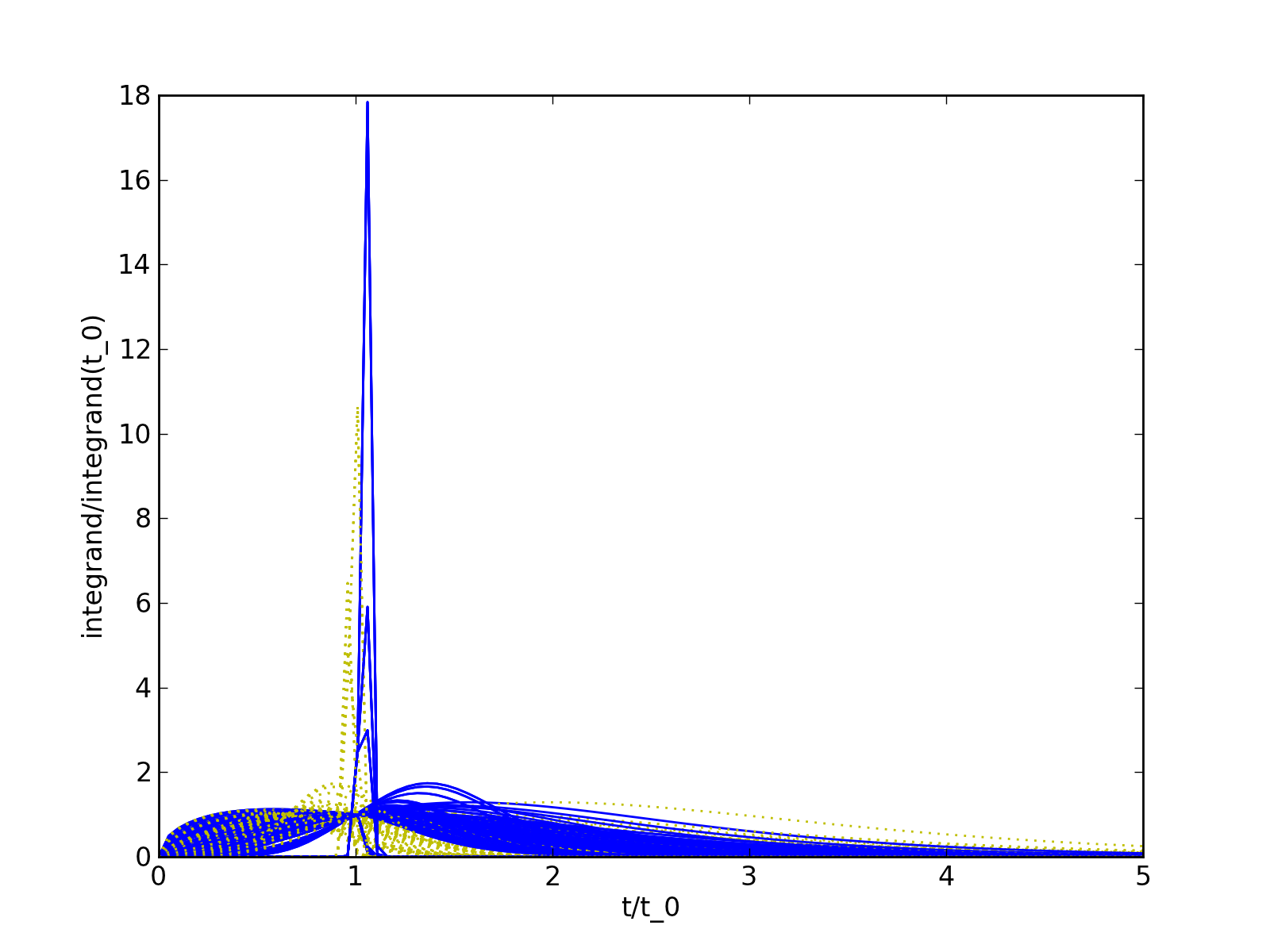
This is known to improve the analytic properties at the endpoints. We
using successively more points until the desired accuracy is
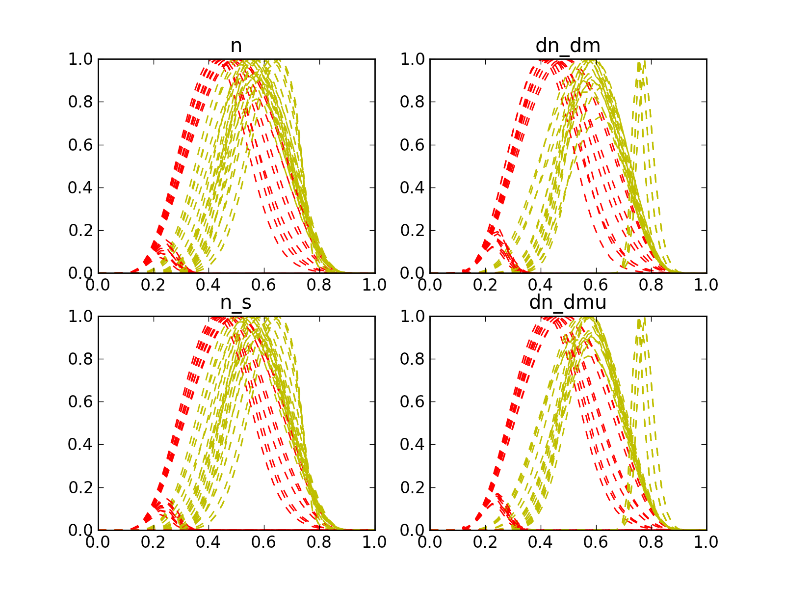
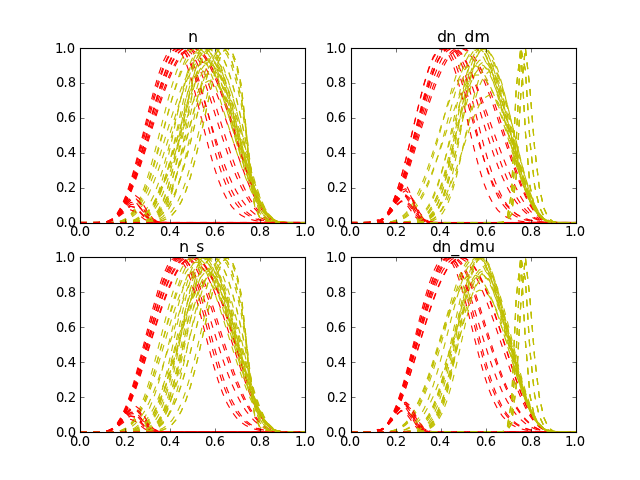
achieved. Here are some examples of the transformed functions as seen
by the trapezoidal method. The yellow curves are for the interval
![[0, k+ \tfrac{1}{2} + \eta]](../_images/math/7e14082573536daaf157a6b38c27377d7516eb5b.png) while the red curves are for the region
while the red curves are for the region
![[k+ \tfrac{1}{2} + \eta, 60\eta]](../_images/math/0455a46b8247d09c2021d64ab4593114130f9a5b.png) .
.
Physical Quantities
Here we present the relevant physical quantities for a single species
of free fermion with mass  and chemical potential
  , and
dispersion
, and
dispersion  . Everything is derived from the
pressure:
. Everything is derived from the
pressure:
System Message: WARNING/2 (\begin{aligned}
P &= \frac{1}{\beta}\int\dbar^{3}{\vect{k}}\;\left[
\ln\left(1+e^{-\beta(E_k-\mu)}\right)
+
\ln\left(1+e^{-\beta(E_k+\mu)}\right)
\right],\\
&= \frac{\sqrt{2}m^4}{3\pi^2}\theta^{5/2}\left[
F_{3/2} + \frac{\theta}{2}F_{5/2}\right]
\end{aligned}
)
latex exited with error:
[stderr]
[stdout]
This is pdfTeX, Version 3.1415926-2.3-1.40.12 (TeX Live 2011)
restricted \write18 enabled.
entering extended mode
(./math.tex
LaTeX2e <2011/06/27>
Babel <v3.8m> and hyphenation patterns for english, dumylang, nohyphenation, ge
rman-x-2011-07-01, ngerman-x-2011-07-01, afrikaans, ancientgreek, ibycus, arabi
c, armenian, basque, bulgarian, catalan, pinyin, coptic, croatian, czech, danis
h, dutch, ukenglish, usenglishmax, esperanto, estonian, ethiopic, farsi, finnis
h, french, friulan, galician, german, ngerman, swissgerman, monogreek, greek, h
ungarian, icelandic, assamese, bengali, gujarati, hindi, kannada, malayalam, ma
rathi, oriya, panjabi, tamil, telugu, indonesian, interlingua, irish, italian,
kurmanji, lao, latin, latvian, lithuanian, mongolian, mongolianlmc, bokmal, nyn
orsk, polish, portuguese, romanian, romansh, russian, sanskrit, serbian, serbia
nc, slovak, slovenian, spanish, swedish, turkish, turkmen, ukrainian, uppersorb
ian, welsh, loaded.
(/usr/local/texlive/2011/texmf-dist/tex/latex/base/article.cls
Document Class: article 2007/10/19 v1.4h Standard LaTeX document class
(/usr/local/texlive/2011/texmf-dist/tex/latex/base/size12.clo))
(/usr/local/texlive/2011/texmf-dist/tex/latex/base/inputenc.sty
(/usr/local/texlive/2011/texmf-dist/tex/latex/ucs/utf8x.def))
(/usr/local/texlive/2011/texmf-dist/tex/latex/ucs/ucs.sty
(/usr/local/texlive/2011/texmf-dist/tex/latex/ucs/data/uni-global.def))
(/usr/local/texlive/2011/texmf-dist/tex/latex/amsmath/amsmath.sty
For additional information on amsmath, use the `?’ option.
(/usr/local/texlive/2011/texmf-dist/tex/latex/amsmath/amstext.sty
(/usr/local/texlive/2011/texmf-dist/tex/latex/amsmath/amsgen.sty))
(/usr/local/texlive/2011/texmf-dist/tex/latex/amsmath/amsbsy.sty)
(/usr/local/texlive/2011/texmf-dist/tex/latex/amsmath/amsopn.sty))
(/usr/local/texlive/2011/texmf-dist/tex/latex/amscls/amsthm.sty)
(/usr/local/texlive/2011/texmf-dist/tex/latex/amsfonts/amssymb.sty
(/usr/local/texlive/2011/texmf-dist/tex/latex/amsfonts/amsfonts.sty))
(/usr/local/texlive/2011/texmf-dist/tex/latex/tools/bm.sty)
(/Users/mforbes/Library/texmf/tex/latex/mmf/mmfmath.sty
(/usr/local/texlive/2011/texmf-dist/tex/latex/mh/mathtools.sty
(/usr/local/texlive/2011/texmf-dist/tex/latex/graphics/keyval.sty)
(/usr/local/texlive/2011/texmf-dist/tex/latex/tools/calc.sty)
(/usr/local/texlive/2011/texmf-dist/tex/latex/mh/mhsetup.sty))
(/usr/local/texlive/2011/texmf-dist/tex/latex/base/ifthen.sty)
(/usr/local/texlive/2011/texmf-dist/tex/latex/doublestroke/dsfont.sty)
(/usr/local/texlive/2011/texmf-dist/tex/generic/mathdots/mathdots.sty))
(/usr/local/texlive/2011/texmf-dist/tex/latex/preview/preview.sty) (./math.aux)
(/usr/local/texlive/2011/texmf-dist/tex/latex/ucs/ucsencs.def)
(/usr/local/texlive/2011/texmf-dist/tex/latex/graphics/graphicx.sty
(/usr/local/texlive/2011/texmf-dist/tex/latex/graphics/graphics.sty
(/usr/local/texlive/2011/texmf-dist/tex/latex/graphics/trig.sty)
(/usr/local/texlive/2011/texmf-dist/tex/latex/latexconfig/graphics.cfg)
(/usr/local/texlive/2011/texmf-dist/tex/latex/graphics/dvips.def)))
Preview: Fontsize 12pt
(/usr/local/texlive/2011/texmf-dist/tex/latex/amsfonts/umsa.fd)
(/usr/local/texlive/2011/texmf-dist/tex/latex/amsfonts/umsb.fd)
! LaTeX Error: Command \dj unavailable in encoding OT1.
See the LaTeX manual or LaTeX Companion for explanation.
Type H <return> for immediate help.
...
l.26 \end{gather}
! LaTeX Error: Command \dj unavailable in encoding OT1.
See the LaTeX manual or LaTeX Companion for explanation.
Type H <return> for immediate help.
...
l.26 \end{gather}
[1] (./math.aux) )
(see the transcript file for additional information)
Output written on math.dvi (1 page, 1128 bytes).
Transcript written on math.log.
The second term is the antiparticle contribution which may or may not
be included. The standard Fermi-Dirac integrals do not include it,
but we will since it is almost always more physical and inexpensive to
include.
The relevant physical quantities follow from differentiating:
Here are the expressions:
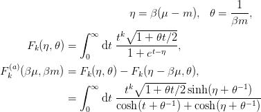
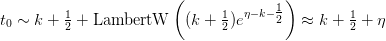
In each case, the behaviour of the integrand is dominated by the
denominator which is minimized at  .
.
Here are some missing intermediate steps:
System Message: WARNING/2 (\begin{aligned}
n_{\beta}(\mu, m)
&= \int \dbar^{3}{k}\;
\frac{1}{1+e^{\beta(\sqrt{k^2 + m^2} - \mu)}}
= \frac{1}{2\pi^2}\int_{0}^{\infty}\d{k}\;
\frac{1}{1+e^{\beta(\sqrt{k^2 + m^2} - \mu)}}
= \left(\frac{m}{2\beta}\right)^{3/2}\frac{2}{\pi^2}
\int_{0}^{\infty}\d{t}\;
\frac{E}{m}\frac{\sqrt{t}\sqrt{1+\theta t/2}}
{1+e^{t-\eta}}.
\end{aligned}
)
latex exited with error:
[stderr]
[stdout]
This is pdfTeX, Version 3.1415926-2.3-1.40.12 (TeX Live 2011)
restricted \write18 enabled.
entering extended mode
(./math.tex
LaTeX2e <2011/06/27>
Babel <v3.8m> and hyphenation patterns for english, dumylang, nohyphenation, ge
rman-x-2011-07-01, ngerman-x-2011-07-01, afrikaans, ancientgreek, ibycus, arabi
c, armenian, basque, bulgarian, catalan, pinyin, coptic, croatian, czech, danis
h, dutch, ukenglish, usenglishmax, esperanto, estonian, ethiopic, farsi, finnis
h, french, friulan, galician, german, ngerman, swissgerman, monogreek, greek, h
ungarian, icelandic, assamese, bengali, gujarati, hindi, kannada, malayalam, ma
rathi, oriya, panjabi, tamil, telugu, indonesian, interlingua, irish, italian,
kurmanji, lao, latin, latvian, lithuanian, mongolian, mongolianlmc, bokmal, nyn
orsk, polish, portuguese, romanian, romansh, russian, sanskrit, serbian, serbia
nc, slovak, slovenian, spanish, swedish, turkish, turkmen, ukrainian, uppersorb
ian, welsh, loaded.
(/usr/local/texlive/2011/texmf-dist/tex/latex/base/article.cls
Document Class: article 2007/10/19 v1.4h Standard LaTeX document class
(/usr/local/texlive/2011/texmf-dist/tex/latex/base/size12.clo))
(/usr/local/texlive/2011/texmf-dist/tex/latex/base/inputenc.sty
(/usr/local/texlive/2011/texmf-dist/tex/latex/ucs/utf8x.def))
(/usr/local/texlive/2011/texmf-dist/tex/latex/ucs/ucs.sty
(/usr/local/texlive/2011/texmf-dist/tex/latex/ucs/data/uni-global.def))
(/usr/local/texlive/2011/texmf-dist/tex/latex/amsmath/amsmath.sty
For additional information on amsmath, use the `?’ option.
(/usr/local/texlive/2011/texmf-dist/tex/latex/amsmath/amstext.sty
(/usr/local/texlive/2011/texmf-dist/tex/latex/amsmath/amsgen.sty))
(/usr/local/texlive/2011/texmf-dist/tex/latex/amsmath/amsbsy.sty)
(/usr/local/texlive/2011/texmf-dist/tex/latex/amsmath/amsopn.sty))
(/usr/local/texlive/2011/texmf-dist/tex/latex/amscls/amsthm.sty)
(/usr/local/texlive/2011/texmf-dist/tex/latex/amsfonts/amssymb.sty
(/usr/local/texlive/2011/texmf-dist/tex/latex/amsfonts/amsfonts.sty))
(/usr/local/texlive/2011/texmf-dist/tex/latex/tools/bm.sty)
(/Users/mforbes/Library/texmf/tex/latex/mmf/mmfmath.sty
(/usr/local/texlive/2011/texmf-dist/tex/latex/mh/mathtools.sty
(/usr/local/texlive/2011/texmf-dist/tex/latex/graphics/keyval.sty)
(/usr/local/texlive/2011/texmf-dist/tex/latex/tools/calc.sty)
(/usr/local/texlive/2011/texmf-dist/tex/latex/mh/mhsetup.sty))
(/usr/local/texlive/2011/texmf-dist/tex/latex/base/ifthen.sty)
(/usr/local/texlive/2011/texmf-dist/tex/latex/doublestroke/dsfont.sty)
(/usr/local/texlive/2011/texmf-dist/tex/generic/mathdots/mathdots.sty))
(/usr/local/texlive/2011/texmf-dist/tex/latex/preview/preview.sty) (./math.aux)
(/usr/local/texlive/2011/texmf-dist/tex/latex/ucs/ucsencs.def)
(/usr/local/texlive/2011/texmf-dist/tex/latex/graphics/graphicx.sty
(/usr/local/texlive/2011/texmf-dist/tex/latex/graphics/graphics.sty
(/usr/local/texlive/2011/texmf-dist/tex/latex/graphics/trig.sty)
(/usr/local/texlive/2011/texmf-dist/tex/latex/latexconfig/graphics.cfg)
(/usr/local/texlive/2011/texmf-dist/tex/latex/graphics/dvips.def)))
Preview: Fontsize 12pt
(/usr/local/texlive/2011/texmf-dist/tex/latex/amsfonts/umsa.fd)
(/usr/local/texlive/2011/texmf-dist/tex/latex/amsfonts/umsb.fd)
! LaTeX Error: Command \dj unavailable in encoding OT1.
See the LaTeX manual or LaTeX Companion for explanation.
Type H <return> for immediate help.
...
l.28 \end{gather}
! LaTeX Error: Command \dj unavailable in encoding OT1.
See the LaTeX manual or LaTeX Companion for explanation.
Type H <return> for immediate help.
...
l.28 \end{gather}
Overfull \hbox (165.30914pt too wide) in paragraph at lines 28–28
[]
[1] (./math.aux) )
(see the transcript file for additional information)
Output written on math.dvi (1 page, 1352 bytes).
Transcript written on math.log.
 . First we note the asymptotic behaviour of the integrand:
 :
: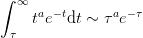
 , then we can neglect the tail for
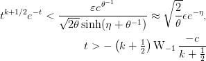
![ct^{k}\sqrt{1 + \tfrac{\theta}{2}t}
\left(
\frac{\cdots}
{\left[\cosh(t + \beta m) + \cosh(\eta + \beta m)\right]^b}
\right)](../_images/math/1e344ac5c3f8c973feef16c51d772fadb4959df7.png)
 :
:

 where
where  is the
distance to the nearest pole and
is the
distance to the nearest pole and  is the step-size. The poles in
the integrand are at must have a step-size of
is the step-size. The poles in
the integrand are at must have a step-size of 
 , we break the interval into two regions
![[0,\eta]](../_images/math/6ba3ace34c4b0e71c5593271ea8556648cc8c473.png) and
and ![[\eta, 60\eta]](../_images/math/4fc394fec4c73536d72d421997aa4e9c15a173c6.png) and use the IMT method which
approximates the integral
and use the IMT method which
approximates the integral
![\begin{aligned}
n &= \pdiff{P}{\mu} \geq 0,\\
n^{(s)} &= -\pdiff{P}{m} \geq 0,\\
n_{,m} &= \pdiff{n}{m} = -n^{(s)}_{,\mu} = -\pdiff{n^{(s)}}{\mu}
= \frac{\partial^{2}P}{\partial\mu \partial m},\\
n_{,\mu} &= \pdiff{n}{\mu} = \pdiff[2]{P}{\mu} \geq 0,\\
n^{(s)}_{,m} &= \pdiff{n^{(s)}}{m} = -\pdiff[2]{P}{m}.
\end{aligned}](../_images/math/96a96d728d27ab11fbb1c7b174361c927aec1cd9.png)
![\begin{aligned}
P &= \frac{(2\beta m)^{3/2}}{6\pi^2 \beta^4}
\int_{0}^{\infty}\d{t}\;\sqrt{1 + \tfrac{\theta}{2}t}
\left(t^{3/2} + \tfrac{\theta}{2} t^{5/2}\right)
\left(\frac{\cosh(\beta\mu) + e^{-(t+\beta m)}}
{\cosh(t + \beta m) + \cosh(\eta + \beta m)}
\right),\\
n &= \frac{(\beta m)^{3/2}}{\sqrt{2}\pi^2 \beta^3}
\int_{0}^{\infty}\d{t}\;\sqrt{1 + \tfrac{\theta}{2}t}
\left(t^{1/2} + \theta t^{3/2}\right)
\left(\frac{\sinh(\beta\mu)}
{\cosh(t + \beta m) + \cosh(\eta + \beta m)}
\right),\\
n^{(s)} &= \frac{(\beta m)^{3/2}}{\sqrt{2}\pi^2 \beta^3}
\int_{0}^{\infty}\d{t}\;\sqrt{1 + \tfrac{\theta}{2}t}
t^{1/2}
\left(\frac{\cosh(\beta\mu) + e^{-(t+\beta m)}}
{\cosh(t + \beta m) + \cosh(\eta + \beta m)}
\right),\\
n_{,\mu} &= \frac{(\beta m)^{3/2}}{\sqrt{2}\pi^2 \beta^2}
\int_{0}^{\infty}\d{t}\;\sqrt{1 + \tfrac{\theta}{2}t}
\left(t^{1/2} + \theta t^{3/2}\right)
\left(\frac{1 + \cosh(t + \beta m)\cosh(\beta\mu)}
{\left[\cosh(t + \beta m) + \cosh(\eta + \beta m)\right]^2}
\right),\\
n^{(s)}_{,\mu} = - n_{,m} &= \frac{(\beta m)^{3/2}}{\sqrt{2}\pi^2 \beta^2}
\int_{0}^{\infty}\d{t}\;\sqrt{1 + \tfrac{\theta}{2}t}
t^{1/2}
\left(\frac{\sinh(t + \beta m)\sinh(\beta\mu)}
{\left[\cosh(t + \beta m) + \cosh(\eta + \beta m)\right]^2}
\right),\\
\end{aligned}](../_images/math/ff9751f9a3279c8265bcc9bf18998a1bbf859281.png)