mmf.physics.seq
| ScarfII(*varargin, **kwargs) | Scarf II (hyperbolic) potential: |
| S(*varargin, **kwargs) | Scarf II (hyperbolic) potential: |
| HO_radial(*varargin, **kwargs) | Radial Harmonic Oscillator. |
| R(x, n, a, b) | Return the Romanovski polynomial |
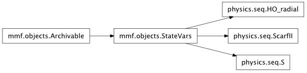
Inheritance diagram for mmf.physics.seq:
Numerical Solutions to the Schrodinger equation.
This module contains some exact solutions to the Schrodinger equation for use in testing.
- class mmf.physics.seq.ScarfII(*varargin, **kwargs)[source]
Bases: mmf.objects.StateVars
Scarf II (hyperbolic) potential:
ScarfII(A=1,
        B=0,
        a=1,
        m=1,
        hbar=1)
![V(x) = \frac{\hbar^2}{2m a^2}\Biggl[A^2 + \left(B^2 - A^2 -
A\right)
\sech^{2}\frac{x}{a} + B\left(2A + 1\right)
\sech\frac{x}{a}\; \tanh \frac{x}{a}\Biggr].](../../../_images/math/daebcd8420d05660f195736084b6321c07e1b886.png)
Notes
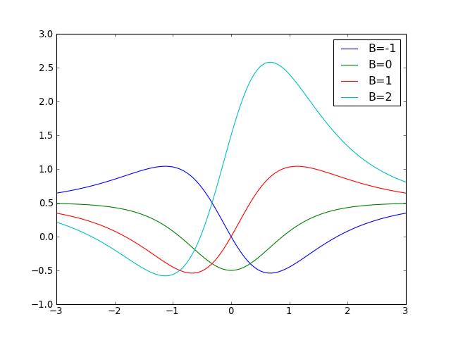
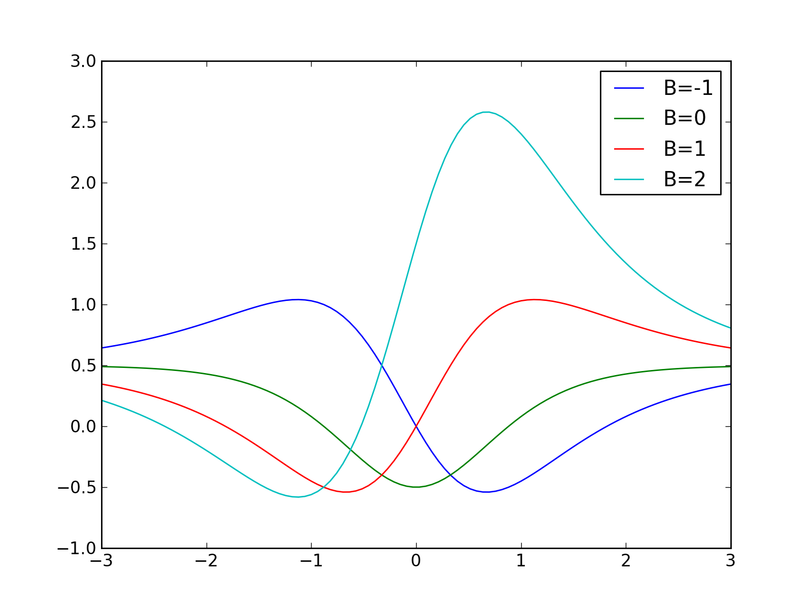
The depth of the potential is controlled by A while the asymmetry is controlled by B (though the spectrum is unchanged).
from mmf.physics.seq import ScarfII
x = np.linspace(-3,3,100)
for B in [-1,0,1,2]:
   V = ScarfII(A=1, B=B)
   plt.plot(x, V(x), label='B=%i'%(B,))

plt.legend()
(Source code, png, hires.png, pdf)

Examples
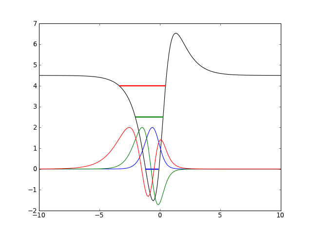
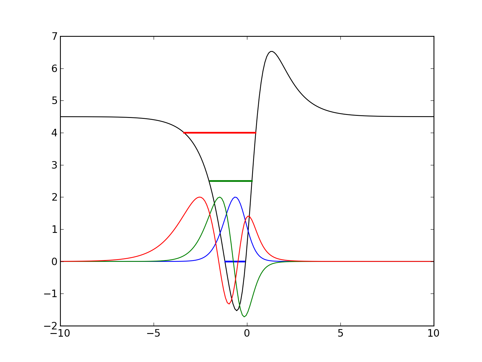
from mmf.physics.seq import ScarfII
V = ScarfII(A=3, B=2)
x = np.linspace(-10, 10, 200)
v = V(x)
En = V.E()
plt.plot(x, v, 'k')
for n, E in enumerate(En):
   x_ = x[np.where(v <= E)][[0, -1]]
   line = plt.plot(x_, x_*0 + E, lw=2)
   colour = line[0].get_color()
   psi = V.psi(n)(x)
   psi = psi/np.max(abs(psi))
   plt.plot(x, 2*psi, colour + '-')
(Source code, png, hires.png, pdf)

Attributes
- class mmf.physics.seq.S(*varargin, **kwargs)[source]
Bases: mmf.objects.StateVars
Scarf II (hyperbolic) potential:
S(A=1,
  B=0,
  a=1,
  m=1,
  hbar=1)
ScarfII(A=1,
        B=0,
        a=1,
        m=1,
        hbar=1)
Notes
The depth of the potential is controlled by A while the asymmetry is controlled by B (though the spectrum is unchanged).
from mmf.physics.seq import ScarfII
x = np.linspace(-3,3,100)
for B in [-1,0,1,2]:
   V = ScarfII(A=1, B=B)
   plt.plot(x, V(x), label='B=%i'%(B,))

plt.legend()
(Source code, png, hires.png, pdf)

Examples
from mmf.physics.seq import ScarfII
V = ScarfII(A=3, B=2)
x = np.linspace(-10, 10, 200)
v = V(x)
En = V.E()
plt.plot(x, v, 'k')
for n, E in enumerate(En):
   x_ = x[np.where(v <= E)][[0, -1]]
   line = plt.plot(x_, x_*0 + E, lw=2)
   colour = line[0].get_color()
   psi = V.psi(n)(x)
   psi = psi/np.max(abs(psi))
   plt.plot(x, 2*psi, colour + '-')
(Source code, png, hires.png, pdf)

Attributes
- hbar
- class mmf.physics.seq.HO_radial(*varargin, **kwargs)[source]
Bases: mmf.objects.StateVars
Radial Harmonic Oscillator.
HO_radial(d=3,
          hbar=1,
          m=1,
          omega=1)
Notes
In d-dimensions, the Hamiltonian is simply a sum over d independent oscillators,
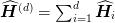 , where each
  is an independent oscillator
in coordinate
is an independent oscillator
in coordinate  . The energies are additive and thus:
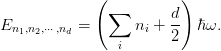
It is useful to consider this as a central potential problem in the coordinate
 . In this case we recover a 1-d problem with
an additional set of quantum numbers corresponding to angular
momentum
. In this case we recover a 1-d problem with
an additional set of quantum numbers corresponding to angular
momentum  . This follows from the expression of the Laplacian
in d-dimensions:
. This follows from the expression of the Laplacian
in d-dimensions: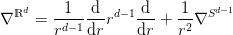
where
 is the Laplacian defined on the unit sphere
 . This can be brought into a simple form by introducing
the radial momentum operator:
. This can be brought into a simple form by introducing
the radial momentum operator:
In terms of this we have:
Finally, introducing the appropriate d-dimensional spherical harmonics
 we have
Combining these gives the effective radial Hamiltonianfootnote{One can define raising a lowering operators to analyse this~cite{Arik:2008ix}.}
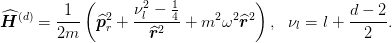
The energy levels
 and degeneracies
  are thus
with normalized radial eigenfunctions are
 where
where
and
 are the generalized Laguerre polynomials.
Attributes
![R_{m}^{(a,b)}(x) &= \frac{1}{w^{(a,b)}(x)}
\diff[m]{}{x}(1+x^2)^{m}w^{(a,b)}(x)\\
w^{(a,b)}(x) &= (1+x^2)^{-a}e^{b\tan^{-1}(x)}](../../../_images/math/aba5bb7c69564fdf3474c32f9f245e4ef4d692ed.png)
![R_{m}^{(a,b)}(x) &= [b + 2(m - a)x]R_{m-1}^{(a,b)}(x)
+ 2(m - 1)(m - a)(1+x^2)R_{m-2}^{(a-1,b)}(x),\\
R_{0}^{(a,b)} &= 1,\\
R_{1}^{(a,b)} &= 2(1-a)x + b.](../../../_images/math/6fac997b53b88cce5ed393c1385e5c16727679cb.png)