mmf.physics.potentials.two_body
| DoubleExponential([v0, r0, mu0, f_v, f_r, ...]) | Double Exponential potential: |
| SoonYongPotential2([v0, A0, V1, A1, hbar, ...]) | Extended Potential used by Soon Yong. |
| Potential([abs_tol, rel_tol, Rmin]) | Instances are callable and return compact potentials V(r). |
| PoschlTeller([v0, r0, hbar, M, abs_tol, ...]) | Extended Poschl-Teller (Rosen-Morse) potential used by Soon |
| BargmannPotential([a, re, hbar, M]) | Bargmann Potential where the effective range expansion is exact |
| PotentialV0R0([abs_tol, rel_tol, Rmin]) | Mixing for two-parameter potentials with a parameter  governing the overall strength and a parameter governing the overall strength and a parameter  governing the effective range. governing the effective range. |
| DoubleGaussian([v0, r0, mu0, f_v, f_r, ...]) | Double Gaussian potential: |
| SoonYongPotential | Extended Poschl-Teller (Rosen-Morse) potential used by Soon |
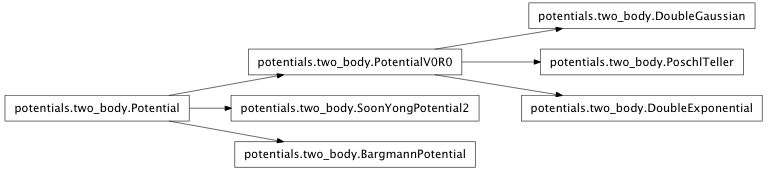
Inheritance diagram for mmf.physics.potentials.two_body:
Code for extracting properties of two-body systems.
Phase Shifts
We consider here short-range potentials such that for  .
In this case, the potential may be described in terms of the phase
shift of the scattering states.
.
In this case, the potential may be described in terms of the phase
shift of the scattering states.
- class mmf.physics.potentials.two_body.DoubleExponential(v0=1.1909151179666313, r0=0.6666666666666666, mu0=None, f_v=-2.0, f_r=2.0, hbar=1.0, M=0.5, abs_tol=1e-12, rel_tol=1e-12, Rmin=0.1)[source]
Bases: mmf.physics.potentials.two_body.PotentialV0R0
Double Exponential potential:
![V(r) = -v_0 \frac{\hbar^2}{M} \mu_0^2 \left(
\exp[-\mu_0 r] + f_v \exp[-\mu_0 r f_r]
\right)](../../../_images/math/277d49f564877716c073a53824aad1f85d1557ea.png)
Note that
 here.
here.>>> v = DoubleExponential(mu0=14.0) >>> v.get_ar() # One of Stefano's values to check. (5852295157..., 0.3099...) >>> v.set_ainv_re(ainv=0.0, re=1.0) >>> v.v0, v.r0 (1.190915117966..., 0.9218838916...)
Methods
__call__(r) compute_R() Return R >= self.Rmin such that `abs(self(R)) < dVdV(r) Return V’(r)/V(r). Should be overloaded for speed and/or gE(E[, R, method]) Return k*cot(delta) as a function of energy E for the specified get_ar([R, method]) Return (a,re) where a is the s-wave scattering length and re is the s-wave effective range. get_deq(f, jac, U0[, method]) Return a “deq” object capable of integrating the system get_deq_E(E[, method]) Return solution to energy dependent differential equation for (u,du) for finding the s-wave phase shift. get_deq_ar([method]) Return the differential equation (u,du,uu,duu) for finding the s-wave scattering length and the s-wave effective range. get_deq_gE(E[, method]) Return solution to energy dependent differential equation get_deq_gE_old(E[, method, version]) Old version in terms of fp and fm. get_mu0() plot([Rmax]) Plot potential. plot_gE(Erange[, Rmax]) Plot potential. plot_u(E[, Rmax]) Plot radial wavefunction. set_ainv_re(ainv, re) Uses a non-linear root-finder to set the parameters v0 and r0 so that the scattering length is 1.0/ainv and the effective range is re. set_mu0(mu0) - __init__(v0=1.1909151179666313, r0=0.6666666666666666, mu0=None, f_v=-2.0, f_r=2.0, hbar=1.0, M=0.5, abs_tol=1e-12, rel_tol=1e-12, Rmin=0.1)[source]
- mu0
- class mmf.physics.potentials.two_body.SoonYongPotential2(v0=-1.0, A0=6.2527, V1=0.0, A1=3.0, hbar=0.15915494309189535, M=0.5, kF=1.0, abs_tol=1e-12, rel_tol=1e-12, Rmin=0.1)[source]
Bases: mmf.physics.potentials.two_body.Potential
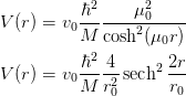
Extended Potential used by Soon Yong.
- V(r) = hbar**2/M*(v0*mu0**2/(cosh(mu0*r))**2
- V1*mu1**2/(cosh(mu1*r))**2)
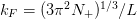
His units are set by kF = (3*pi*pi*N)**(1./3.) / L for a box of length L mu = A*kF
As a test, at unitarity, v0 = 1.0 and re = 2/mu for two-body scattering where m here is the individual mass of the particles.
>>> V = SoonYongPotential2(v0=-1.0,V1=0.0)
>>> (a,re) = V.get_ar()
>>> mu = V.A0*V.kF
>>> abs(a) > 6e8
True
>>> abs(re - 2.0/mu) < 1e-9
True
# kF_SY = (3.*pi)**(2./3.) # EFG_SY = kF_SY**2/2.0*3.0/5.0 # EFG = EFG_SY/4.0/pi**2 # re = 2.0*L/(6.2527*(3.0*pi)**(2./3.)) # # V = -2*hbar^2*mu^2*v0/m/cosh(mu*r)**2 # v0 = 1.0 => ainv = 0, re = 2.0/mu # v0 = 1.30119 => kfa_SY = 1.0
Methods
__call__(r) compute_R() Return R >= self.Rmin such that `abs(self(R)) < dVdV(r) Return V’(r)/V(r). gE(E[, R, method]) Return k*cot(delta) as a function of energy E for the specified get_ar([R, method]) Return (a,re) where a is the s-wave scattering length and re is the s-wave effective range. get_deq(f, jac, U0[, method]) Return a “deq” object capable of integrating the system get_deq_E(E[, method]) Return solution to energy dependent differential equation for (u,du) for finding the s-wave phase shift. get_deq_ar([method]) Return the differential equation (u,du,uu,duu) for finding the s-wave scattering length and the s-wave effective range. get_deq_gE(E[, method]) Return solution to energy dependent differential equation get_deq_gE_old(E[, method, version]) Old version in terms of fp and fm. plot([Rmax]) Plot potential. plot_gE(Erange[, Rmax]) Plot potential. plot_u(E[, Rmax]) Plot radial wavefunction. set_ainv([ainv]) Set the coefficient v0 so that the scattering length is a. set_ainv_re([ainv, re]) Set the coefficients v0 and A0 so that the scattering length is set_ainv_re_VV([ainv, re]) Set the coefficients v0 and V1 so that the scattering length is - __init__(v0=-1.0, A0=6.2527, V1=0.0, A1=3.0, hbar=0.15915494309189535, M=0.5, kF=1.0, abs_tol=1e-12, rel_tol=1e-12, Rmin=0.1)[source]
- dVdV(r)[source]
Return V’(r)/V(r).
V:=v0/cosh(mu0*r)^2+V1/cosh(mu1*r)^2; with(codegen); C(simplify(diff(V,r)/V),optimized);
- set_ainv(ainv=0.0)[source]
Set the coefficient v0 so that the scattering length is a.
>>> V = SoonYongPotential2()
>>> V.v0 = -0.5
>>> V.set_ainv(0.0)
>>> np.allclose(V.v0, -1.0)
True
- set_ainv_re(ainv=0.0, re=0.07)[source]
Set the coefficients v0 and A0 so that the scattering length is 1.0/ainv and the effective range is re.
>>> V = SoonYongPotential2(kF=1.0)
>>> V.V1 = 0.0
>>> V.set_ainv_re(ainv=0.0,re=1.0)
>>> np.allclose(V.A0, 2./V.kF)
True
>>> np.allclose(V.v0, -1.0)
True
- set_ainv_re_VV(ainv=0.0, re=0.07)[source]
Set the coefficients v0 and V1 so that the scattering length is 1.0/ainv and the effective range is re.
>>> V = SoonYongPotential2()
>>> V.A0 = 6.2527
>>> V.A1 = 3.0
>>> V.v0 = -1.5
>>> V.V1 = 0.6
>>> V.set_ainv_re_VV(ainv=0.0,re=0.0)
>>> np.allclose(V.v0, -1.4789900537007772)
True
>>> np.allclose(V.V1, 0.61932931745837538)
True
- class mmf.physics.potentials.two_body.Potential(abs_tol=1e-12, rel_tol=1e-12, Rmin=None)[source]
Bases: object
Instances are callable and return compact potentials V(r).
The class allows one to specify parameters. The important property is that when parameters are modified, the class ensures that the radius returned by R = get_R() is such that V(R) < abs_tol.
The parameter M should be the reduced mass of the system.
Methods
__call__(r) Return V(r). compute_R() Return R >= self.Rmin such that `abs(self(R)) < dVdV(r) Return V’(r)/V(r). Should be overloaded for speed and/or gE(E[, R, method]) Return k*cot(delta) as a function of energy E for the specified get_ar([R, method]) Return (a,re) where a is the s-wave scattering length and re is the s-wave effective range. get_deq(f, jac, U0[, method]) Return a “deq” object capable of integrating the system get_deq_E(E[, method]) Return solution to energy dependent differential equation for (u,du) for finding the s-wave phase shift. get_deq_ar([method]) Return the differential equation (u,du,uu,duu) for finding the s-wave scattering length and the s-wave effective range. get_deq_gE(E[, method]) Return solution to energy dependent differential equation get_deq_gE_old(E[, method, version]) Old version in terms of fp and fm. plot([Rmax]) Plot potential. plot_gE(Erange[, Rmax]) Plot potential. plot_u(E[, Rmax]) Plot radial wavefunction. Construct the potential object.
Methods
__call__(r) Return V(r). compute_R() Return R >= self.Rmin such that `abs(self(R)) < dVdV(r) Return V’(r)/V(r). Should be overloaded for speed and/or gE(E[, R, method]) Return k*cot(delta) as a function of energy E for the specified get_ar([R, method]) Return (a,re) where a is the s-wave scattering length and re is the s-wave effective range. get_deq(f, jac, U0[, method]) Return a “deq” object capable of integrating the system get_deq_E(E[, method]) Return solution to energy dependent differential equation for (u,du) for finding the s-wave phase shift. get_deq_ar([method]) Return the differential equation (u,du,uu,duu) for finding the s-wave scattering length and the s-wave effective range. get_deq_gE(E[, method]) Return solution to energy dependent differential equation get_deq_gE_old(E[, method, version]) Old version in terms of fp and fm. plot([Rmax]) Plot potential. plot_gE(Erange[, Rmax]) Plot potential. plot_u(E[, Rmax]) Plot radial wavefunction. - R
Return a radius for which self(R) <= abs_tol.
- gE(E, R=None, method='odeint')[source]
Return k*cot(delta) as a function of energy E for the specified scattering problem by matching at a specified radius R.
- get_ar(R=None, method='odeint')[source]
Return (a,re) where a is the s-wave scattering length and re is the s-wave effective range. Integrates the wavefunction to radius R. Answer is independent of R if V(r>R) = 0.
- get_deq(f, jac, U0, method='odeint')[source]
Return a “deq” object capable of integrating the system defined by U’ = f(r,U) and diff(U’,U) = jac(r,U) with initial condition U(0.0) = U0.
- get_deq_E(E, method='odeint')[source]
Return solution to energy dependent differential equation for (u,du) for finding the s-wave phase shift.
Uses the following system: du’(r) = 2*m/hbar**2*(V(r)-E)*u(r) u’(r) = du(r)
with initial conditions
u(0) = 0.0 du(0) = 1.0
Call (u,du) = deq.integrate(R) to integrate to R. Note that deq maintains state, so subsequent calls must have increasing R.
This is to be used by calling the method integrate(R).
- get_deq_ar(method='odeint')[source]
Return the differential equation (u,du,uu,duu) for finding the s-wave scattering length and the s-wave effective range.
Uses the following system: u’(r) = du(r) du’(r) = 2*m/hbar**2*V(r)*u(r) uu’(r) = duu(r) duu’(r) = 2*m/hbar**2*(V(r)*uu(r)-u(r))
with initial conditions
u(0) = 0.0 du(0) = 1.0 uu(0) = 0.0 duu(0) = 0.0
Call (u,du,uu,duu) = deq.integrate(R) to integrate to R. Note that deq maintains state, so subsequent calls must have increasing R.
- get_deq_gE(E, method='odeint')[source]
Return solution to energy dependent differential equation for (Ap, Am) for finding the s-wave phase shift which is
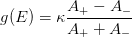
where
 and the s-wave radial wavefunction has the
asymptotic form
and the s-wave radial wavefunction has the
asymptotic form
We solve the radial Schrödinger equation
![u''(r) = [\tilde{V}(r) - \tilde{E}]u(r)](../../../_images/math/aec7d8c4de49e84899a60bd7c63631f8672062cd.png)
where
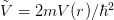 and
and 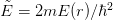 with initial conditions
  , and
, and  using the following
transformation
using the following
transformation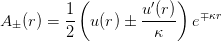
These should be constant at the asymptotic values once
 is larger
than the support of the potential. These functions satisfy the
following set of coupled first-order equations:
is larger
than the support of the potential. These functions satisfy the
following set of coupled first-order equations: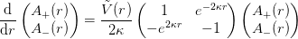
with initial conditions
 .
.
- get_deq_gE_old(E, method='odeint', version=1)[source]
Old version in terms of fp and fm.
version=0
fp' = dfp'
dfp' = (kappa**2 + VV)*fp - V'/V*(kappa*fp - dfp)
fm' = dfm
dfm' = (kappa**2 + VV)*fm + V'/V*(kappa*fm + dfm)

fp(0) = 1/2/kappa
dfp(0) = 1/2
fm(0) = -1/2/kappa
dfm(0) = 1/2
version=1
fp' =  ((2*kappa**2 + VV)*fp + VV*fm)/2/kappa
fm' = -((2*kappa**2 + VV)*fm + VV*fp)/2/kappa

fp(0) = 1/2/kappa
fm(0) = -1/2/kappa
Call (fp,dfp,fm,dfm) = deq.integrate(R) to integrate to R. Note that deq maintains state, so subsequent calls must have increasing R.
This is to be used by calling the method integrate(R).
Examples
>>> V = DoubleGaussian(f_v=0.0)
>>> V._gE_neg(E=-1.0, version=0)
-1.874095805...
>>> V._gE_neg(E=-1.0, version=1)
-1.874095805...
>>> V._gE_neg(E=-1.0, version=2)
-1.874095805...
- class mmf.physics.potentials.two_body.PoschlTeller(v0=-1.0, r0=0.31986181969389227, hbar=1.0, M=0.5, abs_tol=1e-12, rel_tol=1e-12, Rmin=0.1)[source]
Bases: mmf.physics.potentials.two_body.PotentialV0R0
Extended Poschl-Teller (Rosen-Morse) potential used by Soon Yong, Alex, Joe, and Stefano:
Units are set by
 for a box of length
  and
and
 . As a test, at unitarity,
  and
and  for
two-body scattering where
for
two-body scattering where  here is the individual mass of the particles
(M=0.5 by default).
here is the individual mass of the particles
(M=0.5 by default).>>> V = PoschlTeller(v0=-1.0) >>> (a,re) = V.get_ar() >>> mu = 2.0/V.r0 >>> abs(a) > 6e8 True >>> abs(re - 2.0/mu) < 1e-9 True
It is resonant
 for
for 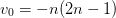 for
for ![n \in [1,2,3,...]](../../../_images/math/84b900a8c2c5b29a5b48cac426fdf2086ca653ea.png) .
.>>> def infty(n): ... return abs(PoschlTeller.a_(-n*(2.0*n-1.0))) >>> infty(1) > 1e8 True >>> infty(2) > 1e8 True
At these resonances one has
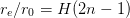 where
where  is the
Harmonic Number
is the
Harmonic Number  .
.>>> def H(n): ... return (1./numpy.arange(1,n+1)).sum() >>> def zero(n): ... return abs(PoschlTeller.re_(-n*(2.0*n-1.0))-H(2*n-1)) >>> zero(1) < 1e-10 True >>> zero(2) < 1e-10 True
The scattering length is zero at the following points where the effective range diverges. I am not sure yet what these correspond to:
v0 = [0.0,-4.4438633257625231,-12.913326147200248,
-25.421577034814653,-41.955714059176017,
-62.508749555456298,...]

# kF_SY = (3.*pi)**(2./3.)
# EFG_SY = kF_SY**2/2.0*3.0/5.0
# EFG = EFG_SY/4.0/pi**2
# re = 2.0*L/(6.2527*(3.0*pi)**(2./3.))
#
# V = -2*hbar^2*mu^2*v0/m/cosh(mu*r)**2
# v0 = 1.0 => ainv = 0, re = 2.0/mu
# v0 = 1.30119 => kfa_SY = 1.0
Methods
__call__(r) compute_R() Return R >= self.Rmin such that `abs(self(R)) < dVdV(r) Return 
gE(E[, R, method]) Return k*cot(delta) as a function of energy E for the specified get_ar([R, method]) Return (a,re) where a is the s-wave scattering length and re is the s-wave effective range. get_deq(f, jac, U0[, method]) Return a “deq” object capable of integrating the system get_deq_E(E[, method]) Return solution to energy dependent differential equation for (u,du) for finding the s-wave phase shift. get_deq_ar([method]) Return the differential equation (u,du,uu,duu) for finding the s-wave scattering length and the s-wave effective range. get_deq_gE(E[, method]) Return solution to energy dependent differential equation get_deq_gE_old(E[, method, version]) Old version in terms of fp and fm. k_cot_delta_analytic(E[, l]) This potential has some analytic properties (see Alex’s thesis and plot([Rmax]) Plot potential. plot_gE(Erange[, Rmax]) Plot potential. plot_u(E[, Rmax]) Plot radial wavefunction. set_ainv([ainv]) Set the coefficient v0 so that the inverse scattering length is ainv. set_ainv_re([ainv, re]) Set the coefficients v0 and r0 so that the inverse scattering length is ainv and the effective range is re. - __init__(v0=-1.0, r0=0.31986181969389227, hbar=1.0, M=0.5, abs_tol=1e-12, rel_tol=1e-12, Rmin=0.1)[source]
- dVdV(r)[source]
Return
V:=v0/cosh(mu0*r)^2+V1/cosh(mu1*r)^2;
with(codegen);
C(simplify(diff(V,r)/V),optimized);
- k_cot_delta_analytic(E, l=None)[source]
This potential has some analytic properties (see Alex’s thesis and references therein):
Examples
>>> V = PoschlTeller(v0=-1.0,r0=2.0/6.2527)
>>> V.gE(E=1.0)
0.1599309...
>>> V.k_cot_delta_analytic(E=1.0)
0.1599309...
- class mmf.physics.potentials.two_body.BargmannPotential(a=1.0, re=0.4, hbar=0.15915494309189535, M=0.5, **kwarg)[source]
Bases: mmf.physics.potentials.two_body.Potential
Bargmann Potential where the effective range expansion is exact with only a and r_e.
>> V = BargmannPotential(a=1.0,re=0.01) >> (a,re) = V.get_ar() >> (a,re) (1.0, 0.1)
Methods
__call__(r) compute_R() Return R >= self.Rmin such that `abs(self(R)) < dVdV(r) Return V’(r)/V(r). gE(E[, R, method]) Return k*cot(delta) as a function of energy E for the specified get_ar([R, method]) Return (a,re) where a is the s-wave scattering length and re is the s-wave effective range. get_deq(f, jac, U0[, method]) Return a “deq” object capable of integrating the system get_deq_E(E[, method]) Return solution to energy dependent differential equation for (u,du) for finding the s-wave phase shift. get_deq_ar([method]) Return the differential equation (u,du,uu,duu) for finding the s-wave scattering length and the s-wave effective range. get_deq_gE(E[, method]) Return solution to energy dependent differential equation get_deq_gE_old(E[, method, version]) Old version in terms of fp and fm. plot([Rmax]) Plot potential. plot_gE(Erange[, Rmax]) Plot potential. plot_u(E[, Rmax]) Plot radial wavefunction.
- class mmf.physics.potentials.two_body.PotentialV0R0(abs_tol=1e-12, rel_tol=1e-12, Rmin=None)[source]
Bases: mmf.physics.potentials.two_body.Potential
Mixing for two-parameter potentials with a parameter
governing the
overall strength and a parameter governing the effective range. The
potential can have additional parameters, but these two will be adjusted to
set the scattering-length and range.Methods
__call__(r) Return V(r). compute_R() Return R >= self.Rmin such that `abs(self(R)) < dVdV(r) Return V’(r)/V(r). Should be overloaded for speed and/or gE(E[, R, method]) Return k*cot(delta) as a function of energy E for the specified get_ar([R, method]) Return (a,re) where a is the s-wave scattering length and re is the s-wave effective range. get_deq(f, jac, U0[, method]) Return a “deq” object capable of integrating the system get_deq_E(E[, method]) Return solution to energy dependent differential equation for (u,du) for finding the s-wave phase shift. get_deq_ar([method]) Return the differential equation (u,du,uu,duu) for finding the s-wave scattering length and the s-wave effective range. get_deq_gE(E[, method]) Return solution to energy dependent differential equation get_deq_gE_old(E[, method, version]) Old version in terms of fp and fm. plot([Rmax]) Plot potential. plot_gE(Erange[, Rmax]) Plot potential. plot_u(E[, Rmax]) Plot radial wavefunction. set_ainv_re(ainv, re) Uses a non-linear root-finder to set the parameters v0 and r0 so that the scattering length is 1.0/ainv and the effective range is re. Construct the potential object.
Methods
__call__(r) Return V(r). compute_R() Return R >= self.Rmin such that `abs(self(R)) < dVdV(r) Return V’(r)/V(r). Should be overloaded for speed and/or gE(E[, R, method]) Return k*cot(delta) as a function of energy E for the specified get_ar([R, method]) Return (a,re) where a is the s-wave scattering length and re is the s-wave effective range. get_deq(f, jac, U0[, method]) Return a “deq” object capable of integrating the system get_deq_E(E[, method]) Return solution to energy dependent differential equation for (u,du) for finding the s-wave phase shift. get_deq_ar([method]) Return the differential equation (u,du,uu,duu) for finding the s-wave scattering length and the s-wave effective range. get_deq_gE(E[, method]) Return solution to energy dependent differential equation get_deq_gE_old(E[, method, version]) Old version in terms of fp and fm. plot([Rmax]) Plot potential. plot_gE(Erange[, Rmax]) Plot potential. plot_u(E[, Rmax]) Plot radial wavefunction. set_ainv_re(ainv, re) Uses a non-linear root-finder to set the parameters v0 and r0 so that the scattering length is 1.0/ainv and the effective range is re. - __init__(abs_tol=1e-12, rel_tol=1e-12, Rmin=None)
Construct the potential object.
- class mmf.physics.potentials.two_body.DoubleGaussian(v0=0.7860976072874742, r0=0.6666666666666666, mu0=None, f_v=-4.0, f_r=2.0, hbar=1.0, M=0.5, abs_tol=1e-12, rel_tol=1e-12, Rmin=0.1)[source]
Bases: mmf.physics.potentials.two_body.PotentialV0R0
Double Gaussian potential:
![V(r) &= -v_0 \frac{\hbar^2}{M} \mu_0^2 \left(
\exp[-(\mu_0 r/2)^{2}] + f_v \exp[-(\mu_0 r f_r/2)^2]
\right)\\
&= -v_0 \frac{\hbar^2}{M} \mu_0^2 \left(
\exp[-(\mu_0 r/2)^{2}] + f_v \exp[-(\mu_0 r f_r/2)^2]
\right)\\](../../../_images/math/c8567b520e372aadc5107ad00e896fbb951b622d.png)
Note that
here.>>> v = DoubleGaussian(mu0=12.0) >>> v.get_ar() # One of Stefano's values to check. (-2887043864..., 0.3293...) >>> v.set_ainv_re(ainv=0.0, re=1.0) >>> v.v0, v.r0 (0.786097607..., 1.012180386...)
Methods
__call__(r) compute_R() Return R >= self.Rmin such that `abs(self(R)) < dVdV(r) Return V’(r)/V(r). Should be overloaded for speed and/or gE(E[, R, method]) Return k*cot(delta) as a function of energy E for the specified get_ar([R, method]) Return (a,re) where a is the s-wave scattering length and re is the s-wave effective range. get_deq(f, jac, U0[, method]) Return a “deq” object capable of integrating the system get_deq_E(E[, method]) Return solution to energy dependent differential equation for (u,du) for finding the s-wave phase shift. get_deq_ar([method]) Return the differential equation (u,du,uu,duu) for finding the s-wave scattering length and the s-wave effective range. get_deq_gE(E[, method]) Return solution to energy dependent differential equation get_deq_gE_old(E[, method, version]) Old version in terms of fp and fm. get_mu0() plot([Rmax]) Plot potential. plot_gE(Erange[, Rmax]) Plot potential. plot_u(E[, Rmax]) Plot radial wavefunction. set_ainv_re(ainv, re) Uses a non-linear root-finder to set the parameters v0 and r0 so that the scattering length is 1.0/ainv and the effective range is re. set_mu0(mu0) - __init__(v0=0.7860976072874742, r0=0.6666666666666666, mu0=None, f_v=-4.0, f_r=2.0, hbar=1.0, M=0.5, abs_tol=1e-12, rel_tol=1e-12, Rmin=0.1)[source]
- mu0
- mmf.physics.potentials.two_body.SoonYongPotential
alias of PoschlTeller