`mmf.math.ode.deq`¶

`bvp`
`SympyODE`(varargin, *kwargs)	Represent an ODE.
`IDict`(v, *kw)
`Solution`(varargin, *kwargs)	Represents the solution to an ODE as returned by colnew. The default version simply ensures that copies are made of the abscissa because the colnew solution will mutate these.
`Transform`	Abscissa tranformation objects should honour this interface.
`log_transform`(r0, r1, rS)	Implements a logarithmic transform of z in [0, 1] to [r0, r1]
`ODE`(varargin, *kwargs)	Base class to simplify the interface to colnew.
`ODE_1_2`(varargin, *kwargs)	Simplified ODE interface for a single second order allowing for

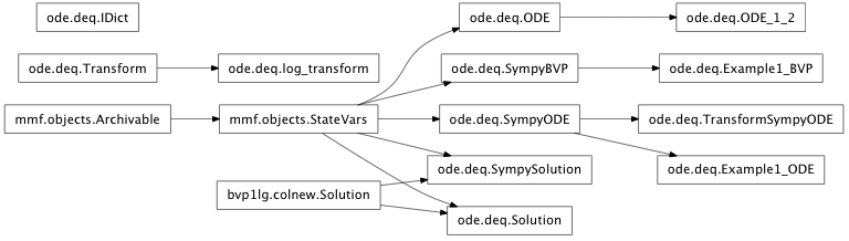
Inheritance diagram for mmf.math.ode.deq:

Inheritance diagram of mmf.math.ode.deq

Interface to 1D colnew ode solver.

Overview¶

Here we provide a simplified interface to the colnew boundary value solver. This can solve differential equations for a set of functions $Y_i(x)$ of the form

$Y_i^{(m_i)} = f_i(x, Z)$

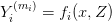
where

$Z = [&[Y_1, Y_1', \ldots, Y_1^{(m_1-2)}, Y_1^{(m_1-1)}],\\ &[Y_2, Y_2', \ldots, Y_2^{(m_2-1)}],\\ &[\ldots],\\ &[Y_n, Y_n', \ldots, Y_n^{(m_n-3)}, Y_n^{(m_n-2)}, Y_n^{(m_n-1)}]]$

is the set of derivatives $Y^{(m)} = \d^{m}{Y}(x)/\d{x}^m$ . Thus, there are $n$ differential equations of orders $m_1$ , $m_2$ , $\ldots$ , $m_n`$ .

Note

Constants may be implemented using $m=1$ equations with $Y'= 0$ in which case $Y$ is a constant to be found. Likewise, if one of the constraints is that an integrated quantity has a fixed value (total particle number for example), then you can introduce $N(x)$ through the first order equation $N'(x) = n(x)$ and give the boundary conditions $N(0)=0$ and $N(x_{\text{max}}) = N$ . These two techniques are often used together to implement the constraint $N$ with a Lagrange multiplier $\mu$ that is entered as a constant parameter.

The m_star = m_1 + m_2 + ... m_n boundary conditions are specified by the conditions

$g_j(y_j, Z) = 0$

at boundary points $a_l \leq x_1 \leq x_2 \leq \cdots x_{m^*} \leq a_r$ . (In these formula, the abscissa $x_j$ is implicit.) The solution will be tabulated on the range $x\in [a_l, a_r]$ .

To simplify the interface, it is assumed that the user will give names to the n variables Y_n and define the functions f_(Y_n).

Debugging Tips:

Try solving a related problem of the same for, but with a known exact solution! If you give this as a guess, then you should get the answer. It is also invaluble to use an exact solution to check all of the functions to make sure there are no coding mistakes.
If you get a SingularCollocationMatrix: Singular collocation matrix in COLNEW error, then try commenting out the derivative functions d_* by adding an underscore _d_*. This way, colnew will compute these using finite differences. This is slow, but will catch typo’s!
Set verbosity to a higher value.
Backoff from singular points until things work, then approach them.
Add print statements to the various functions to print out parameters and x values. You might find that things are getting singular.
Try setting self.problem_regularity = 1. This makes colnew more careful.
Note: The plotting function executes in a try block (to prevent plotting errors from killing the solution). This can catch KeyboardInterrupt... You might have to press Ctr-C many times while plotting...

Transformations¶

Any system can be reduced to a system of first-order equations by introducing auxiliary variables for the higher orders. I.e. for $u''(x) = f(x, u, u'(x))$ one can introduce $v(x) = u'(x)$ to express this as the system

$v'(x) = f(x, u, v)\\ u'(x) = v.$

Let us combine all variables into a single vector $x_i$ so that the system becomes (the first equation is trivial $x_0 \equiv x$ so $x_0' = 1$ )

$\d{x_i} = f_i(\vect{x})\d{x}$

Now express these in terms of new variables as functions $x_i(y_j)$ . The resulting differentials satisfy

$\d{x_i} = \sum_j \pdiff{x_{i}}{y_{j}}\d{y_j} = \sum_j J_{ij}y_j$

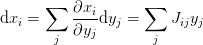
where $J_{ij}$ is the Jacobian of the transformation. We may thus write

$\d{y_i} = \sum_j J^{-1}_{ij} \d{x_j} = \sum_j J^{-1}_{ij} f_j\d{x}$

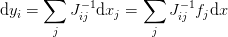
Dividing with $\d{y_0}$ , we obtain

$y'_a = \frac{\sum_j J^{-1}_{aj} f_j}{\sum_j J^{-1}_{0j} f_j}.$

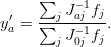
Everything on the right-hand-side can be expressed in terms of the new variables.

class mmf.math.ode.deq.SympyODE(*varargin, **kwargs)¶

Bases: mmf.objects.StateVars

Represent an ODE.

SympyODE(vars=Required,
         eqs=Required,
         bcs=Required,
         params={})

Specify the original ODE here in terms of the original variables either as a string or using :pkg:`sympy`. The :pkg:`sympy` package will be used to define the various functions required to satisfy the BVP interface.

Examples

>>> class Example1(SympyODE):
...     _state_vars = [
...         ('vars', ['x', 'u', 'v']),
...         ('eqs',
...          ['-u(x).diff(x)/x + ((nu/x)**2 -1)*u(x) - u(x).diff(x,x)',
...           'x**(nu+1)*u(x) - v(x).diff(x)']),
...         ('bcs',
...          [(1, 1e-5, 'u(x) - besselj(nu,x)'),
...           (10, 0, 'u(x) - besselj(nu,x)'),
...           (5, 1e-5, 'v(x) - x**(nu+1)*besselj(nu+1,x)')]),
...         ('nu', 3.4123)]
...     process_vars()
>>> e = Example1()
>>> s = e.solve(maximum_mesh_size=300)

Attributes

State Variables:
`vars`¶	List of sympy vars [x, Y_1, Y_2, ..., Y_n], the first of which is the abscissa, and the rest correspond to the variables Y_i.
`eqs`¶	List of equations defining the system. Each equation should be zero – i.e. the lhs of $Y^{(m)} - f(x, Z) = 0$ – and linear in the highest derivative.
`bcs`¶	List of tuples [(x, g)] where xs = [x_1, x_2, ...] is the set of abscissa for the boundary conditions, and gs = [g_1(x,Z), g_2(x,Z), ...] is the list of equations. Note: the boundary points xs must evaluate to numbers (they cannot contain parameters), the equations gs should explicitly contain the abscissa (to allow later for transformations), but the equations gs are not permitted to have the highest derivative. The xs need not be sorted.
`params`¶	Dictionary of parameter values. The equations can be expressed in terms of additional constants. One can specify values here, or define them directly as state variables. (This dictionary allows you to avoid possible name-clashes.) These values will be preferred if a parameter appears both here and as a state var.

Methods

`all_items`()	Return a list [(name, obj)] of (name, object) pairs containing all items available.
`archive`(name)	Return a string representation that can be executed to restore the object.
`archive_1`([env])	Return (rep, args, imports).
`initialize`(**kwargs)	Calls `__init__()` passing all assigned attributes.
`items`([archive])	Return a list [(name, obj)] of (name, object) pairs where the
`resume`()	Resume calls to `__init__()` from `__setattr__()`,
`suspend`()	Suspend calls to `__init__()` from

This is the initialization routine. It is called after the attributes specified in _state_vars have been assigned.

The user version should perform any after-assignment initializations that need to be performed.

Note

Since all of the initial arguments are listed in kwargs, this can be used as a list of attributes that have “changed” allowing the initialization to be streamlined. The default __setattr__() method will call __init__() with the changed attribute to allow for recalculation.

This recomputing only works for attributes that are assigned, i.e. iff __setattr__() is called. If an attribute is mutated, then __getattr__() is called and there is no (efficient) way to determine if it was mutated.

Computed values with True Computed.save will be passed in through kwargs when objects are restored from an archive. These parameters in general need not be recomputed, but this opens the possibility for an inconsistent state upon construction if a user inadvertently provides these parameters. Note that the parameters still cannot be set directly.

See __init__() Semantics for details.

Methods

`all_items`()	Return a list [(name, obj)] of (name, object) pairs containing all items available.
`archive`(name)	Return a string representation that can be executed to restore the object.
`archive_1`([env])	Return (rep, args, imports).
`initialize`(**kwargs)	Calls `__init__()` passing all assigned attributes.
`items`([archive])	Return a list [(name, obj)] of (name, object) pairs where the
`resume`()	Resume calls to `__init__()` from `__setattr__()`,
`suspend`()	Suspend calls to `__init__()` from

__init__(*varargin, **kwargs)¶

This is the initialization routine. It is called after the attributes specified in _state_vars have been assigned.

The user version should perform any after-assignment initializations that need to be performed.

Note

Since all of the initial arguments are listed in kwargs, this can be used as a list of attributes that have “changed” allowing the initialization to be streamlined. The default __setattr__() method will call __init__() with the changed attribute to allow for recalculation.

This recomputing only works for attributes that are assigned, i.e. iff __setattr__() is called. If an attribute is mutated, then __getattr__() is called and there is no (efficient) way to determine if it was mutated.

Computed values with True Computed.save will be passed in through kwargs when objects are restored from an archive. These parameters in general need not be recomputed, but this opens the possibility for an inconsistent state upon construction if a user inadvertently provides these parameters. Note that the parameters still cannot be set directly.

See __init__() Semantics for details.

class mmf.math.ode.deq.IDict(*v, **kw)[source]¶

Bases: dict

Methods

`clear`	D.clear() -> None. Remove all items from D.
`copy`	D.copy() -> a shallow copy of D
`fromkeys`(...)	v defaults to None.
`get`	D.get(k[,d]) -> D[k] if k in D, else d. d defaults to None.
`has_key`	D.has_key(k) -> True if D has a key k, else False
`items`	D.items() -> list of D’s (key, value) pairs, as 2-tuples
`iteritems`	D.iteritems() -> an iterator over the (key, value) items of D
`iterkeys`	D.iterkeys() -> an iterator over the keys of D
`itervalues`	D.itervalues() -> an iterator over the values of D
`keys`	D.keys() -> list of D’s keys
`notify_update`()
`pop`	D.pop(k[,d]) -> v, remove specified key and return the corresponding value.
`popitem`	D.popitem() -> (k, v), remove and return some (key, value) pair as a
`setdefault`	D.setdefault(k[,d]) -> D.get(k,d), also set D[k]=d if k not in D
`update`	D.update([E, ]**F) -> None. Update D from dict/iterable E and F.
`values`	D.values() -> list of D’s values
`viewitems`	D.viewitems() -> a set-like object providing a view on D’s items
`viewkeys`	D.viewkeys() -> a set-like object providing a view on D’s keys
`viewvalues`	D.viewvalues() -> an object providing a view on D’s values

__init__(*v, **kw)[source]¶

notify_update()[source]¶

class mmf.math.ode.deq.Solution(*varargin, **kwargs)[source]¶

Bases: mmf.objects.StateVars, scikits.bvp1lg.colnew.Solution

Represents the solution to an ODE as returned by colnew. The default version simply ensures that copies are made of the abscissa because the colnew solution will mutate these.

Solution(ispace=Required,
         fspace=Required,
         ode=Required)

Attributes

class mmf.math.ode.deq.Transform[source]¶

Bases: object

Abscissa tranformation objects should honour this interface.

Methods

`rdot`(x)	Return the derivative dr/dx evaluated at x.
`rdot_r`(r)	Return the derivative dr/dx evaluated at r.
`x`(r)	Return x(r), the inverse transformation.

__init__()¶: x.__init__(...) initializes x; see help(type(x)) for signature

rdot(x)[source]¶: Return the derivative dr/dx evaluated at x.

rdot_r(r)[source]¶: Return the derivative dr/dx evaluated at r.

x(r)[source]¶: Return x(r), the inverse transformation. Should lie in [0, 1].

class mmf.math.ode.deq.log_transform(r0, r1, rS)[source]¶

Bases: mmf.math.ode.deq.Transform

Implements a logarithmic transform of z in [0, 1] to [r0, r1] with typical scale rS at r0.

Methods

`rdot`(x)
`rdot_r`(r)
`x`(r)

Transformation from [0, 1] to [r0, r1] with scale rS at r0.

Methods

`rdot`(x)
`rdot_r`(r)
`x`(r)

__init__(r0, r1, rS)[source]¶: Transformation from [0, 1] to [r0, r1] with scale rS at r0.

rdot(x)[source]¶

rdot_r(r)[source]¶

x(r)[source]¶

class mmf.math.ode.deq.ODE(*varargin, **kwargs)[source]¶

Bases: mmf.objects.StateVars

Base class to simplify the interface to colnew.

ODE(Solution=<class 'mmf.math.ode.deq.Solution'>,
    left=None,
    right=None,
    maximum_mesh_size=1000,
    problem_regularity=0,
    verbosity=0,
    coarsen_initial_guess_mesh=True,
    plot=False,
    plot_pause=0,
    _debug=False)

Attributes

class mmf.math.ode.deq.ODE_1_2(*varargin, **kwargs)[source]¶

Bases: mmf.math.ode.deq.ODE

Simplified ODE interface for a single second order allowing for transformations.

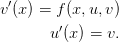
Original Equation: y’‘(x) = f(x, y, y’)

Transformation: x = s(a) y = t(b)

Transformed system: Q’(a) = f(s(a), t(b), Q)/s’(a) b’(a) = s’(a)/t’(b)*Q(a)

This class requires you to define your Example: A’‘(x) = 2*(A(x) + x*A’(x)) A(-1) = 1 A(2) = exp(3)

Solution: A(x) = exp(x**2-1)

Attributes

`collocation_points`
`extra_fixed_points`

Methods

`all_items`()	Return a list [(name, obj)] of (name, object) pairs containing all items available.
`archive`(name)	Return a string representation that can be executed to restore the object.
`archive_1`([env])	Return (rep, args, imports).
`boundary_conditions`(j, mu, **kwargs)	This function must return the j‘th boundary condition(s), which should be zero if and only if the boundary condition(s) at x = self.boundary_point[j] is satsified.
`boundary_points`	Default value for required attributes.
`check_sol`(sol)	This function should check the solution sol, possibly
`initialize`(**kwargs)	Calls `__init__()` passing all assigned attributes.
`items`([archive])	Return a list [(name, obj)] of (name, object) pairs where the
`plotter`(idict, **kwargs)	Default plotter.
`resume`()	Resume calls to `__init__()` from `__setattr__()`,
`solve`([sol])	Return solution.
`suspend`()	Suspend calls to `__init__()` from
`vars`	Default value for required attributes.

This is the initialization routine. It is called after the attributes specified in _state_vars have been assigned.

The user version should perform any after-assignment initializations that need to be performed.

Note

Since all of the initial arguments are listed in kwargs, this can be used as a list of attributes that have “changed” allowing the initialization to be streamlined. The default __setattr__() method will call __init__() with the changed attribute to allow for recalculation.

This recomputing only works for attributes that are assigned, i.e. iff __setattr__() is called. If an attribute is mutated, then __getattr__() is called and there is no (efficient) way to determine if it was mutated.

Computed values with True Computed.save will be passed in through kwargs when objects are restored from an archive. These parameters in general need not be recomputed, but this opens the possibility for an inconsistent state upon construction if a user inadvertently provides these parameters. Note that the parameters still cannot be set directly.

See __init__() Semantics for details.

Attributes

`collocation_points`
`extra_fixed_points`

Methods

`all_items`()	Return a list [(name, obj)] of (name, object) pairs containing all items available.
`archive`(name)	Return a string representation that can be executed to restore the object.
`archive_1`([env])	Return (rep, args, imports).
`boundary_conditions`(j, mu, **kwargs)	This function must return the j‘th boundary condition(s), which should be zero if and only if the boundary condition(s) at x = self.boundary_point[j] is satsified.
`boundary_points`	Default value for required attributes.
`check_sol`(sol)	This function should check the solution sol, possibly
`initialize`(**kwargs)	Calls `__init__()` passing all assigned attributes.
`items`([archive])	Return a list [(name, obj)] of (name, object) pairs where the
`plotter`(idict, **kwargs)	Default plotter.
`resume`()	Resume calls to `__init__()` from `__setattr__()`,
`solve`([sol])	Return solution.
`suspend`()	Suspend calls to `__init__()` from
`vars`	Default value for required attributes.

__init__(*varargin, **kwargs)¶

This is the initialization routine. It is called after the attributes specified in _state_vars have been assigned.

The user version should perform any after-assignment initializations that need to be performed.

Note

Since all of the initial arguments are listed in kwargs, this can be used as a list of attributes that have “changed” allowing the initialization to be streamlined. The default __setattr__() method will call __init__() with the changed attribute to allow for recalculation.

This recomputing only works for attributes that are assigned, i.e. iff __setattr__() is called. If an attribute is mutated, then __getattr__() is called and there is no (efficient) way to determine if it was mutated.

Computed values with True Computed.save will be passed in through kwargs when objects are restored from an archive. These parameters in general need not be recomputed, but this opens the possibility for an inconsistent state upon construction if a user inadvertently provides these parameters. Note that the parameters still cannot be set directly.

See __init__() Semantics for details.

Table Of Contents

Previous topic

This Page

`mmf.math.ode.deq`¶

Overview¶

Transformations¶

Navigation

Table Of Contents

Previous topic

This Page

Quick search

mmf.math.ode.deq¶

Overview¶

Transformations¶

Navigation

`mmf.math.ode.deq`¶