mmf.math.interp

UnivariateSpline(x, y[, w, bbox, k, s])	Representation of spline functions based on scipy.interpolate.fitpack.splrep().
EvenUnivariateSpline(x, y[, w, bbox, k, s])	Representation of spline functions for even functions.
InterpolatedUnivariateSpline(x, y[, k, bbox])	Interpolated univariate spline approximation.
Options(*varargin, **kwargs)	Class of options supported by the tabulate function and Interpolate class.
NoRefinement	Exception signalling no refinement.
TolMet	Exception signalling no refinement because tolerance met.
Discontinuity	Exception signalling no refinement because a possible
DegenerateRefinement	Exception signalling no refinement because refinement would
Interpolator(*varargin, **kwargs)	Represents an interpolation of a function.
Rbf(*v, **kw)	My wrapper for scipy.interpolate.Rbf that supports
RectBivariateSpline(x, y, z[, bbox, kx, ky, s])	Replacement that allows derivatives to be computed.
get_score(value, err, abs_tol, rel_tol)	Return the score of an error.
tabulate(f, xmin, xmax, opt[, interp])	Return an interpolation object representing the function f to
interp_mat(x0, x1[, k])	Return the interpolation matrix and its pseudo-inverse that linearly interpolate functions from the basis x0 to x1 and back.

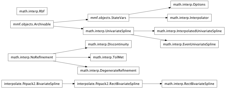
Inheritance diagram for mmf.math.interp:

Interpolation library for use with scipy. This library provides several tools for interpolating and approximating functions in multiple dimensions.

One challange with an interpolation is to quantify the errors of the interpolation. In other words: “How good is the interpolation”. If the function is never particularly small, the appropriate measure is most often the relative error (f_i-f)/f. If f becomes small, however, then this may diverge. Below some threshold |f| < f_c, the more appropriate measure of the error is the absolute error f_i - f.

Tolerances should thus always be specified as a pair: abs_tol and rel_tol. The threshold is f_c = abs_tol/rel_tol.

We thus define the score:

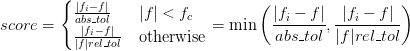
If both abs_tol and rel_tol are zero, then the score is 1 + |f_i - f|. In this way scores greater than 1 mean that the specified tolerances are not met.

A drawback to this approach, however, is that it is not possible to specify the errors of an interpolation that crosses zero without specifying the threshhold f_c. The maximum absolute error may always be given, and the maximum relative error will have meaning if f is never too close to zero. An interesting number is the value f_abs_rel of f at which the relative errors become of order unity. Thus, the error will be characterized by a quadruplet:

(max_score, max_abs_err, max_rel_err, f_abs_rel)

class mmf.math.interp.UnivariateSpline(x, y, w=None, bbox=[None, None], k=3, s=None)

Bases: mmf.objects.Archivable

Representation of spline functions based on scipy.interpolate.fitpack.splrep().

Does a few things extra:

• Fixes bug that changes the shape of arguments.
• Ensures that all input points are used as knots (to prevent smoothing from simplifying the knots and possibly changing the parity of the functions.)
• Allows for inputs to be unsorted.
• Allows for y to be the output of a vectorized function. The last index corresponds to the vector x.

Examples

>>> import numpy as np
>>> x = np.linspace(0,2*np.pi,10)
>>> np.random.seed(0)
>>> y0 = np.cos(x) + 0.01*np.random.rand(10)
>>> y1 = np.sin(x) + 0.01*np.random.rand(10)
>>> spline = UnivariateSpline(x=x, y=[y0,y1], k=3, s=0.0)
>>> X = np.linspace(0, 2*np.pi, 100)
>>> Y = np.array([np.cos(X), np.sin(X)])
>>> dY = np.array([-np.sin(X), np.cos(X)])
>>> np.allclose(Y, spline(X), atol=0.02)
True
>>> np.allclose(dY, spline(X, nu=1), atol=0.06)
True

>>> x = np.random.rand(10)
>>> y = x**3
>>> spline = UnivariateSpline(x=x,y=y,k=3,s=0.0)
>>> X = np.random.rand(100)
>>> Y = X**3
>>> np.allclose(spline(X), Y)
True

Methods

archive(name)	Return a string representation that can be executed to restore the object.
archive_1([env])	Return (rep, args, imports).
integral(a, b)	Return definite integral of the spline between two
items()	Return list of data to make the object archivable.
roots()	Return the zeros of the spline.
set_smoothing_factor(s)	Continue spline computation with the given smoothing

__init__(x, y, w=None, bbox=[None, None], k=3, s=None)

integral(a, b)

Return definite integral of the spline between two given points.

items()

Return list of data to make the object archivable.

roots()

Return the zeros of the spline.

Restriction: only cubic splines are supported by fitpack.

set_smoothing_factor(s)

Continue spline computation with the given smoothing factor s and with the knots found at the last call.

class mmf.math.interp.EvenUnivariateSpline(x, y, w=None, bbox=[None, None], k=3, s=None)

Bases: mmf.math.interp.UnivariateSpline

Representation of spline functions for even functions.

Assumes that the data represents an even function and extends the knots to make sure that the spline is even.

Does a few things extra:

• Fixes bug that changes the shape of arguments.
• Ensures that all input points are used as knots (to prevent smoothing from simplifying the knots and possibly changing the parity of the functions.)

Methods

archive(name)	Return a string representation that can be executed to restore the object.
archive_1([env])	Return (rep, args, imports).
integral(a, b)	Return definite integral of the spline between two
items()	Return list of data to make the object archivable.
roots()
set_smoothing_factor(s)	Continue spline computation with the given smoothing

__init__(x, y, w=None, bbox=[None, None], k=3, s=None)

integral(a, b)

Return definite integral of the spline between two given points.

roots()

class mmf.math.interp.InterpolatedUnivariateSpline(x, y, k=None, bbox=[None, None])

Bases: mmf.math.interp.UnivariateSpline

Interpolated univariate spline approximation.

Based on scipy class, but with some sugar to allow for unsorted inputs etc. and to make it archivable.

Examples

>>> s = InterpolatedUnivariateSpline([2, 1, 3], [4, 1, 9], k=2)
>>> print s
InterpolatedUnivariateSpline(x=[2, 1, 3], y=[4, 1, 9], bbox=[None, None], k=2)
>>> ld = {}
>>> exec(s.archive('s'), ld)
>>> ld['s']
InterpolatedUnivariateSpline(x=[2, 1, 3], y=[4, 1, 9], bbox=[None, None], k=2)

Methods

archive(name)	Return a string representation that can be executed to restore the object.
archive_1([env])	Return (rep, args, imports).
integral(a, b)	Return definite integral of the spline between two
items()	Return list of data to make the object archivable.
roots()	Return the zeros of the spline.
set_smoothing_factor(s)	Continue spline computation with the given smoothing

Parameters :

x : array

A 1d array of x values. Must be unique. (Need not be sorted.)

y : array

An nd array of y values to be interpolated. Must have

y.shape[-1] == len(x).

k : int

Order of b-splines (1<=k<=5)

Methods

archive(name)	Return a string representation that can be executed to restore the object.
archive_1([env])	Return (rep, args, imports).
integral(a, b)	Return definite integral of the spline between two
items()	Return list of data to make the object archivable.
roots()	Return the zeros of the spline.
set_smoothing_factor(s)	Continue spline computation with the given smoothing

__init__(x, y, k=None, bbox=[None, None])

Parameters :

x : array

A 1d array of x values. Must be unique. (Need not be sorted.)

y : array

An nd array of y values to be interpolated. Must have

y.shape[-1] == len(x).

k : int

Order of b-splines (1<=k<=5)

class mmf.math.interp.Options(*varargin, **kwargs)

Bases: mmf.objects.StateVars

Class of options supported by the tabulate function and Interpolate class.

Options(algorithm=expensive,
        abs_tol=1e-08,
        rel_tol=1e-08,
        x_tol=0.0,
        n_min=6,
        n_max=100,
        n_new=1,
        maxTime=inf,
        k=3,
        groupSize=10,
        linear_refinement=True,
        weighted=False,
        plot=False,
        plot_N=1000,
        plot_exact=False,
        plot_spline=True,
        verbose=False,
        xy=None,
        guess=None)

Attributes

State Variables:
algorithm	Either ‘cheap’ or ‘expensive’. The latter is better for very expensive functions, because it tries to choose the best possible interval each time. If there are many points, however, this is very expensive. Thus, only use the ‘expensive’ option if you need a few very well placed points.
abs_tol	The algorithm halts if the function is approximated to within this absolute tolerance. This means that if you remove a tabulated point from the data and use the rest to define an interpolating spline, then the spline will interpolate the removed point with an absolute error of less than abs_tol. Of course, there is always a risk that the spline will miss highly local features, but it does a pretty good job.
rel_tol	If the function magnitude is large, then the tolerance is placed on the relative error rather than the absolute error.
x_tol	The minimum spacing of the sample points.
n_min	Minimum number of samples.
n_max	Maximum number of points. For the ‘expensive’ algorithm, the program stops after this many points. The ‘cheap’ algorithm may overshoot by a factor of two before stopping.
n_new	Number of new intervals to try to fix each step.
maxTime	The maximum elapsed time before the algorithm halts. The ‘expensive’ algorithm may overshoot by a single function evaluation and some processing. The ‘cheap’ algorithm may overshoot by up to N function evaluations (where there are N points in the current approximation).
k	The order of the interpolating b-spline. k=3 works well for most smooth functions.
groupSize	This is only relevant for the ‘expensive’ algorithm. Instead of only taking the worst interval each time and then recalculating the splines, the worst groupSize intervals are tabulated. If the function is not too expensive to compute, then this can significantly speed up the algorithm.
linear_refinement	If this is true, the refinements are made based on the errors of a linear (k==1) interpolation. Such an interpolation is much faster than using the full spline unless special properties of the spline are used. (It is possible to use a special form of cubic spline to efficiently evaluate the knot_errors, but I only know how to do this with a radial basis function formulation which is not efficient or accurate for spline computations as the matrices are ill-conditioned and not tri-diagonal.)
weighted	If true, the expensive algorithm places the midpoints closer to the point with the worse score. If false, then the midpoints are used.
plot	If plot>0 then the results will be plotted as the program runs. This includes the tabulated points and the interpolating spline. Intermediate calculations are also plotted if plot>1 (only applicable if groupSize>1 or using ‘cheap’ algorithm).
plot_N	Number of (equally spaced) points to add to the spline.
plot_exact	Display also the exact function for comparison when plotting spline.
plot_spline	If true, plot the spline as well as the sample points. If false, only plot the tabulation points.
verbose	If true, then each iteration is reported (errors etc.)
xy	Tuple (xi, y) of arrays allow you to supply data if you already have computed it. This will be used in the initial tabulation and will reduce the number of points computed (only n_min points are computed before the algorithm starts working.)
guess	If this is a string, then an interpolated guess will be passed to the function as f(guess=...) to provide an initial guess. Especially useful if f implements an iterative scheme.

Methods

all_items()	Return a list [(name, obj)] of (name, object) pairs containing all items available.
archive(name)	Return a string representation that can be executed to restore the object.
archive_1([env])	Return (rep, args, imports).
initialize(**kwargs)	Calls __init__() passing all assigned attributes.
items([archive])	Return a list [(name, obj)] of (name, object) pairs where the
resume()	Resume calls to __init__() from __setattr__(),
suspend()	Suspend calls to __init__() from

Verify that the arguments are reasonable.

Methods

all_items()	Return a list [(name, obj)] of (name, object) pairs containing all items available.
archive(name)	Return a string representation that can be executed to restore the object.
archive_1([env])	Return (rep, args, imports).
initialize(**kwargs)	Calls __init__() passing all assigned attributes.
items([archive])	Return a list [(name, obj)] of (name, object) pairs where the
resume()	Resume calls to __init__() from __setattr__(),
suspend()	Suspend calls to __init__() from

__init__(*varargin, **kwargs)

Verify that the arguments are reasonable.

class mmf.math.interp.NoRefinement

Bases: exceptions.Exception

Exception signalling no refinement.

__init__()

x.__init__(...) initializes x; see help(type(x)) for signature

class mmf.math.interp.TolMet

Bases: mmf.math.interp.NoRefinement

Exception signalling no refinement because tolerance met.

__init__()

x.__init__(...) initializes x; see help(type(x)) for signature

class mmf.math.interp.Discontinuity

Bases: mmf.math.interp.NoRefinement

Exception signalling no refinement because a possible discontinuity has been found.

__init__()

x.__init__(...) initializes x; see help(type(x)) for signature

class mmf.math.interp.DegenerateRefinement

Bases: mmf.math.interp.NoRefinement

Exception signalling no refinement because refinement would yield degenerate abscissa.

__init__()

x.__init__(...) initializes x; see help(type(x)) for signature

class mmf.math.interp.Interpolator(*varargin, **kwargs)

Bases: mmf.objects.StateVars

Represents an interpolation of a function. This is the heart of the algorithm. It provides a mechanism for determining a good adaptive set of sample points to provide a good interpolating representation of the function.

Interpolator(x=Required,
             y=Required,
             new_x=[])

Attributes

class mmf.math.interp.Rbf(*v, **kw)

Bases: object

My wrapper for scipy.interpolate.Rbf that supports vectorization.

Parameters :

x, y, ... : array-like

One-dimensional arrays specifying the abscissa points that define the interpolation. Each of these must have the same length N.

f(x, y,...) : array-like

The last positional argument should be the data. It may have any shape as long as the last dimension has length N. The interpolation will be (inefficiently) vectorized over the shape.

Examples

Here we simultaneously interpolate two functions over the plane:

>>> import numpy as np    
>>> def f(x, y):
...     r2 = x*x + y*y
...     return np.array([np.sin(2*x*y)*np.exp(-r2),
...                      x*np.cos(3*x**2+y)*np.exp(-r2)])
>>> np.random.seed(0)
>>> x = np.random.rand(100)
>>> y = np.random.rand(100)
>>> f12 = f(x,y)
>>> f12.shape
(2, 100)
>>> rbf = Rbf(x, y, f12)
>>> rbf = Rbf([x, y], f12)  # Can also stack x and y
>>> np.allclose(rbf(x,y), f(x,y))
True
>>> X, Y = np.mgrid[-0.1:1.1:10j,-0.1:1.1:10j]
>>> abs_err = abs(rbf(X,Y) - f(X,Y))
>>> rel_err = abs(abs_err/f(X,Y))
>>> err = np.minimum(abs_err, rel_err)
>>> err.max() < 0.18
True

The choice of axis ordering here is to facilitate usage with broadcasting functions like f as defined above. Another common use is with tabulated values. This will require some transposes:

>>> f12 = np.array([f(_x, _y) for (_x, _y) in zip(x,y)]).T
>>> f12.shape
(2, 100)
>>> rbf = Rbf(x, y, f12)
>>> np.allclose(rbf(x,y), f12)
True

__init__(*v, **kw)

class mmf.math.interp.RectBivariateSpline(x, y, z, bbox=[None, None, None, None], kx=3, ky=3, s=0)

Bases: scipy.interpolate.fitpack2.RectBivariateSpline

Replacement that allows derivatives to be computed. See ticket #1522.

Methods

ev(xi, yi)	Evaluate spline at points (x[i], y[i]), i=0,...,len(x)-1
get_coeffs()	Return spline coefficients.
get_knots()	Return a tuple (tx,ty) where tx,ty contain knots positions of the spline with respect to x-, y-variable, respectively.
get_residual()	Return weighted sum of squared residuals of the spline
integral(xa, xb, ya, yb)	Evaluate the integral of the spline over area [xa,xb] x [ya,yb].

__init__(x, y, z, bbox=[None, None, None, None], kx=3, ky=3, s=0)

mmf.math.interp.get_score(value, err, abs_tol, rel_tol)

Return the score of an error. If score <= 1 then the specified tolerances have been met. The tolerances are met if either rel_err <= rel_tol or abs(err) < abs_tol.

If both abs_tol and rel_tol are zero, the score is 1 + abs(err).

Examples

>>> get_score(1, 0.1, 0.1, 0.001)
array([ 1.])
>>> get_score(1, 0.2, 0.1, 0.001)
array([ 2.])
>>> get_score(200, 0.2, 0.1, 0.001)
array([ 1.])
>>> get_score(200, 0.2, 0, 0)
array([ 1.2])

mmf.math.interp.tabulate(f, xmin, xmax, opt, interp=None)

Return an interpolation object representing the function f to with tolerance tol over the interval [xmin, xmax]

Parameters :

f : function

Function to approximate y = f(x). If the function can accept an initial guess (to seed an iteration for example), then an interpolated guess will be passed if opt.guess is set to the name of the argument. (I.e. if opt.guess = ‘y0’, then the function will be called as f(x, y0=...)). No argument will be passed if an interpolation cannot be formed: it is up to the function to provide an initial guess.

If the function fails to compute a value, then it should throw a ValueError exception. In the output, x and y will contain such points, but they will not be used in the extrapolation. The output xflag will contain ones where the points have been succesfully computed.

xmin, xmax : float

Range of interpolation.

Note

Make sure the function is not antisymmetric over this interval: this can really mess up the tabulation because the inner interpolation will always go through zero, causing an underestimation in the error of the central intervals!

opt : Options

Options instance containing control parameters.

interp : :

Previous interpolation. Will be used as a starting point.

Notes

The algorithm works by sampling at least n_min points (including initial data if provided). Then the points are given a “score” by evaluating max(abs(y - ys)) where ys is the interpolated value using the spline fit through all points except the current point. Each interval is given a”score” which is the average of the scores of the endpoints.

The ‘expensive’ algorithm computes the function at a point in the worst opt.groupSize intervals. If the weighted option is chosesn, then midpoint is closer to the endpoint with the worst score. This can help the algorithm approach new features, but does not fill in the function as well and can miss features. Use this if your function is extremely ‘expensive’ to compute.

The ‘cheap’ algorithm proceeds to compute new points at all midpoints specified by the previous iteration, and then checks to see how well the new midpoints are fit by the spline through the old points. The intervals next to points who’s score is less than the tolerance are then used in the next iteration.

This is repeted until one of the termination criteria is reached.

The primary diference is that, once new points are added, the spline will change, affecting the scores of neighbouring intervals. The cheap algorithm ignores this effect which minimizes the number of spline computations while the expensive algorithm recomputes the spline each time. The ‘cheap’ algorithm computes one spline and up to N new points per iteration whereas the expensive algorithm computes N splines per iteration and only up to opt.groupSize new points per iteration.

The advantage of the expensive algorithm is that a new point might indicate a large deviation from the current spline, signaling a new feature (like a peak). The ‘expensive’ algorithm will then start sampling points around this feature. The ‘cheap’ algorithm will first fill out all of the previous subintervals before it attempts to analyze the new feature.

Examples

>>> import numpy as np
>>> opt = Options()
>>> tabulate(np.sin, 0, 1, opt)(0.4) 
0.389418...

If you have some previous values, you can use these:

>>> x0 = np.linspace(0,1,10)
>>> opt.xy = (x0, np.sin(x0))
>>> tabulate(np.sin, 0, 1, opt)(0.4) 
0.389418...

mmf.math.interp.interp_mat(x0, x1, k=3)

Return the interpolation matrix and its pseudo-inverse that linearly interpolate functions from the basis x0 to x1 and back.

Parameters :

x0, x1 : array

Interpolate from x0 to x1.

k : int, optional

Order of spline. 1 <= k <= 5. Default k=3 is recommended.

Notes

The motivation for this is the fixed-point problem:

where f(x) is some fairly smooth function on the real line. I might try and solve this problem on a fixed set of abscissa where I represent the function as a vector . The fixed-point problem is now formulated on this discrete space,

and I can form the Jacobian:

Suppose I have a coarse solution and now want to interpolate this to a finer mesh with some interpolation:

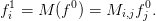
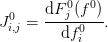
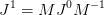
How does the Jacobian transform? If we view the coordinate transformation as. In general, we want a formula of the type:

however, as M is usually rank deficient, there is ambiguity in pseudo-inverse. Here we just use the standard pseudo-inverse, but one might like to consider this choice in the future.

Examples

>>> import numpy as np
>>> x0 = np.linspace(0,1,100)
>>> x1 = np.linspace(0,1,200)
>>> M, Minv = interp_mat(x0,x1)
>>> f0 = np.sin(x0)
>>> f1 = np.dot(M, f0)
>>> np.max(abs(f1 - np.sin(x1))) < 5e-10
True