mmf.math.integrate.integrate_1d.quadrature
| Decay | Represents information about the asymptotic form of indefinite integrals. |
| PowerDecay(x, n[, x0]) | Represents a power-law decay. |
| ExpDecay(x, b[, x0]) | Represents an exponential decay. |
| IntegrationError([mesg, res, err]) | Error during integration. |
| get_weights(x, roots[, cond]) | Return the list of weights wx for quadratures of increasing |
| get_weights_y(x, y, wy) | Return the weights wx for a quadrature of order at least n >= len(y) for the abscissa x give the n exact quadrature abscissa y and weights wy defining a quadrature of order 2n. |
| integrate(f, a, b[, abs_tol, rel_tol, ...]) | Return (res, err) where res is the integral of the function f(x) from a to b and err is an estimate of the absolute error. |
| quad(f, a, b, *varargin, **kwargs) | An improved version of integrate.quad that does some argument checking and deals with points properly. |
| mquad(f, a, b[, abs_tol, verbosity, fa, fb, ...]) | Return (res, err) where res is the numerically evaluated |
| h_roots(n) | Return the abscissa and weights for the Gaussian quadrature of |
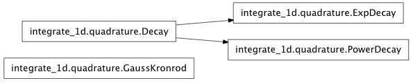
Inheritance diagram for mmf.math.integrate.integrate_1d.quadrature:
Adaptive quadrature routines for one-dimensional integrals.
This module provides access to several adaptive quadrature routines for performing one-dimensional integrals. The main routine is integrate(), which performs a one-dimensional integral. It allows the user to specify properties of the integrand to facilitate an accurate computation.
In particular, the nature of the decay at inf can be described by using a subclass of Decay such as PowerDecay or ExpDecay to effect a transformation for dealing with these tails.
Orthogonal Polynomials
Here we review some properties of orthogonal polynomials and define
notations that are useful for quadratures. We consider polynomials
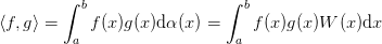
orthogonal to some measure  and define the induced
inner product:
and define the induced
inner product:
Formally we shall work with orthonormal polynomials  –
–
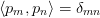 – though the standard
representations
– though the standard
representations  typically are not normalized:
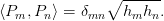
The polynomials are characterized in terms of the coefficients
 ,
,  ,
,  ,
,  ,
,  , and
, and
 ; and the functions
  ,
,  , and
, and
 . In addition, for a given degree
  , one has
quadrature abscissa
, one has
quadrature abscissa  – which are the roots of
 – and weights
  :
:
![&P_{n+1} = (a_n x + b_n) P_n - c_n P_{n-1},\\
&h_n = \braket{P_n,P_n},\\
&Q(x)P_n'' + L(x)P_n' + \lambda_n P_n = 0,\\
&P_n = \frac{1}{e_n W(x)}\diff[n]{}{x}[W(x)Q^{n}(x)],\\
&p_n(x_{n;i}) = 0,\\
&\int_{a}^{b} f(x)W(x)\d{x} = \sum_i w_{n;i} f(x_{n;i})](../../../_images/math/0cbd22061ad6397619ff50f72d383d09ad802b5e.png)
where the last integral is exact for polynomials  of
degree
of
degree  or less. The weights are sometimes
called the “Christoffel Numbers” and may be denoted
or less. The weights are sometimes
called the “Christoffel Numbers” and may be denoted  .
Additional useful relationships are
.
Additional useful relationships are
![&\begin{aligned}
P_n &= k_n x^n + k'_n x^{n-1} + \cdots, &
a_n &= \frac{k_{n+1}}{k_{n}}, &
b_n &= a_n\left(\frac{k'_{n+1}}{k_{n+1}}
- \frac{k'_{n}}{k_{n}}\right), &
c_n &= a_n\frac{k_{n-1}h_{n}}{k_{n}h_{n-1}}
\end{aligned},\\
&R(x) = W(x)Q(x) = \exp\left(\int\frac{L(x)}{Q(x)}\d{x}\right),\\
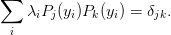
&\sum_{i=0}^{n-1} w_{n;i}p_j(x_{n;i})p_k(x_{n;i}) = \delta_{jk}
\quad \forall j,k < n,\\
&w_{n;i} = \int_{a}^{b}
\left[\frac{p_n(x)}{(x-x_{n;i}) p'_n(x)}\right]^2\d{\alpha(x)}
= -\frac{h_n}{p_{n+1}(x_i)p'_n(x_i)}](../../../_images/math/54ef7ad6a131d837c0388f4f28ca9044134bdbe2.png)
Todo
Check formulae for the weights with h_roots() which seems to work.
Here we summarize some of the known and useful analytic results:
| Name |  |
|
|
|
|
|
|
|
|
|
|---|---|---|---|---|---|---|---|---|---|---|
| Hermite |  |
 |
2 | 0 | 2n |  |
 |
2n | 1 | -2x |
| Laguerre |  |
 |
 |
 |
 |
 |
 |
n | x |  |
Quadrature Formulae
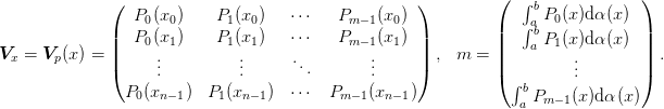
The general idea of a quadrature is to express an integral as
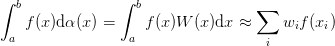
where is a weighting function,  are a set
of weights and
are a set
of weights and  are a set of abscissa. In general, given
weights and abscissa, we have degrees of
freedom, and so we can in general choose these so that the integral is
exact for special forms of : Typically, polynomials of
degree . Since the quadrature is linear, this is realized
through the equations:
are a set of abscissa. In general, given
weights and abscissa, we have degrees of
freedom, and so we can in general choose these so that the integral is
exact for special forms of : Typically, polynomials of
degree . Since the quadrature is linear, this is realized
through the equations:
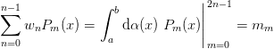
where  is the m‘th moment of the degree m polynomial
 . (One can simply use
  but the
system is typically somewhat better conditioned if one chooses
orthogonal polynomials).
but the
system is typically somewhat better conditioned if one chooses
orthogonal polynomials).
If the abscissa are given, we can determine the weights to satisfy
 “normal” equations through the linear system. We start with
the problem of determining the weights for a given set of abscissa.
We want as high an order as possible, but with all the weights being
positive. (One can relax this somewhat by formally minimizing
“normal” equations through the linear system. We start with
the problem of determining the weights for a given set of abscissa.
We want as high an order as possible, but with all the weights being
positive. (One can relax this somewhat by formally minimizing
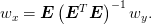
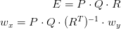
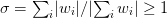 to minimize
roundoff error from cancellation when computing the integral.) One
strategy might be to solve as many equations as possible while
minimizing the norm of w. This leads to the solution
to minimize
roundoff error from cancellation when computing the integral.) One
strategy might be to solve as many equations as possible while
minimizing the norm of w. This leads to the solution
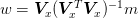
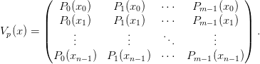
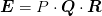
where is the vector of moments and  is the incomplete
Vandermonde matrix at the points
is the incomplete
Vandermonde matrix at the points  :
:
If there is an all positive solution, then this will be all positive. To see this, consider the singular value decomposition of mat{X}:
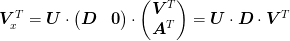
We may write the solution as

where the projection of w in the subspace spanned by  is fixed by the equation and the projection in the complementary
subspace spanned by
is fixed by the equation and the projection in the complementary
subspace spanned by  is arbitrary (
 ).
The set of all valid w spans a linear subspace. With a little thought
about this in lower dimensions, one can convince oneself that if any
points lie within the given “quadrant” of positive w, then the point
closest to the origin will satisfy this (i.e. the point w with
minimal norm). This is the solution with
).
The set of all valid w spans a linear subspace. With a little thought
about this in lower dimensions, one can convince oneself that if any
points lie within the given “quadrant” of positive w, then the point
closest to the origin will satisfy this (i.e. the point w with
minimal norm). This is the solution with  which is
given by the normal equation above.
which is
given by the normal equation above.
Note
This assumes some properties about the nature of the set of solutions that are typically true for the integration problem with reasonable (positive) weights. This should be clarified at some point.
This formula is acceptable only for low orders, otherwise the
Vandermonde matrix quickly becomes ill-conditioned. A better solution
is to use a robust algorithm such as that in Demmel and Koev,
“Accurate SVDs of polynomial Vandermonde matrices involving
orthonormal polynomials”, Linear Algebra and its Applications 411
(2006) 382–396. There they point out that the Vandermonde matrix we
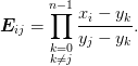
need  can be expressed in
terms of the square Vandermonde matrix
can be expressed in
terms of the square Vandermonde matrix  where
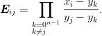
where  are the roots of
  for the order n orthogonal polynomial through the Lagrange
interpolation formula
for the order n orthogonal polynomial through the Lagrange
interpolation formula
For classical orthogonal polynomials, the roots can be
accurately calculated from the recurrence relationships (see below).
Some algebra shows that our weights can be expressed in terms of the
classical weights as
This can also be directly computed from the SVD or QR decompositions
of  . As pointed out in A. J. Cox and N. J. Higham,
“Stability of Householder QR factorization for weighted least squares
problems”, Numerical Analysis 1997 (Dundee), Pitman Res. Notes
Math. Ser. 380, pp. 57–73, Longman, Harlow, 1998, if we first sort
the rows in order of decreasing
. As pointed out in A. J. Cox and N. J. Higham,
“Stability of Householder QR factorization for weighted least squares
problems”, Numerical Analysis 1997 (Dundee), Pitman Res. Notes
Math. Ser. 380, pp. 57–73, Longman, Harlow, 1998, if we first sort
the rows in order of decreasing  norm, then the
standard implementation of the QR decomposition is stable. We do this
in pqr(). Thus:
norm, then the
standard implementation of the QR decomposition is stable. We do this
in pqr(). Thus:
This requires the following knowledge:
The Vandermonde matrix should be formed from orthogonal polynomials
 :
:
Note that one can scale out the weights if needed, so this is not an arduous requirement in most cases.
The algorithm requires the roots
of the highest order
 :
:
The algorithm requires the Christoffel numbers
 :
:
Here is an example of abscissa for integrals between 0 and 1.
>>> def m_(n):
...     return 1./(np.arange(n).reshape((n,1))+1)
>>> def X_(x,n):
...     return x**np.arange(n).reshape((n,1))
>>> def w(x,n):
...     X = np.mat(X_(x,n))
...     l = np.linalg.solve(X*X.T, m_(n))
...     return X.T*l
As an example, let’s consider order two quadratures over the interval [0,1] containing the endpoints and one interior point. An analysis of Simpsons rule shows that positive weights exist if the midpoint lies between 1/3 and 2/3:
>>> np.min(w(np.array([0,0.9/3,1]),3))
-0.0555555555...
>>> round(np.min(w(np.array([0,1/3,1]),3)),14)
0.0
>>> np.min(w(np.array([0,1/2,1]),3))
0.1666666...
>>> round(np.min(w(np.array([0,2/3,1]),3)),14)
0.0
>>> np.min(w(np.array([0,2.1/3,1]),3))
-0.055555555555...
Now, suppose we have
- class mmf.math.integrate.integrate_1d.quadrature.Decay[source]
Bases: float
Represents information about the asymptotic form of indefinite integrals.
Methods
as_integer_ratio() -> (int, int) Returns a pair of integers, whose ratio is exactly equal to the original float and with a positive denominator. conjugate Returns self, the complex conjugate of any float. fromhex((string) -> float) Create a floating-point number from a hexadecimal string. hex float.hex() -> string is_integer Returns True if the float is an integer. - __init__()
x.__init__(...) initializes x; see help(type(x)) for signature
- class mmf.math.integrate.integrate_1d.quadrature.PowerDecay(x, n, x0=0)[source]
Bases: mmf.math.integrate.integrate_1d.quadrature.Decay
Represents a power-law decay.
The function should behave as

where this behaviour becomes dominant for
 .
.Parameters : n : float
Power of decay

x0 : float
Point beyond which decay is the dominant behaviour. This must have the same sign as the value (and must not be zero).
Notes
The transformation used maps
 to
to
 .
.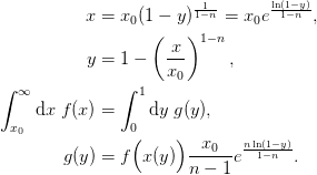
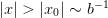
If
 as
as  ,
then
,
then  approaches a constant as
  which is very easy to integrate.
Examples
>>> f = lambda p:1./(p**2 + 1)
>>> a = PowerDecay(-np.inf, x0=-1.0, n=2)
>>> b = PowerDecay(np.inf, x0=1.0, n=2)
>>> a.y_x(a.x_y(0.5))
0.5
>>> a.y_x(-1.0)
0.0
>>> b.y_x(1.0)
0.0
>>> quad(f, -np.inf, -1.0)
(0.785398163397448..., 1.2888...e-10)
>>> quad(a.get_g(f), a.y_x(-np.inf), a.y_x(-1.0))
(0.785398163397448..., 8.7196...e-15)
>>> quad(f, 1.0, np.inf)
(0.785398163397448..., 1.2888...e-10)
>>> quad(b.get_g(f), b.y_x(1.0), b.y_x(np.inf))
(0.785398163397448..., 8.71967...e-15)
This is what integrate does automatically:
>>> integrate(f, a, -1.0)
(0.785398163397448..., 8.71967...e-15)
>>> integrate(f, 1.0, b)
(0.785398163397448..., 8.71967...e-15)
Methods
as_integer_ratio() -> (int, int) Returns a pair of integers, whose ratio is exactly equal to the original float and with a positive denominator. conjugate Returns self, the complex conjugate of any float. fromhex((string) -> float) Create a floating-point number from a hexadecimal string. get_g(f) Return the function g(y) which, when integrated over hex float.hex() -> string is_integer Returns True if the float is an integer. x_y(y) Return x(y) where  and
andy_x(x) Return y(x) where and
 .
.- class mmf.math.integrate.integrate_1d.quadrature.ExpDecay(x, b, x0=None)[source]
Bases: mmf.math.integrate.integrate_1d.quadrature.Decay
Represents an exponential decay.
The function should behave as
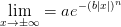
where this behaviour becomes dominant for
 .
.Parameters : b : float
Length-scale: i.e. decay of form

x0 : float
Point beyond which decay is the dominant behaviour. This must have the same sign as the value. If not specified, then it is set to 1/b
Notes
The transformation used maps
to
yin[0,1).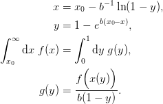
Examples
>>> f = lambda p:3/np.sqrt(np.pi)/(np.exp((3.0*p)**2))
>>> a = ExpDecay(-np.inf, b=3)
>>> b = ExpDecay(np.inf, b=3)
>>> a.y_x(a.x_y(0.5))
0.5...
>>> a.y_x(-3.0)
0.0
>>> b.y_x(3.0)
0.0
>>> quad(f, -np.inf, 0)
(0.49999999..., 2.2113658...e-09)
>>> quad(a.get_g(f), a.y_x(-np.inf), a.y_x(0))
(0.5000000..., 1.177...e-09)
This is what integrate does automatically:
>>> integrate(f, a, 0)
(0.5, 4.8318...e-13)
Methods
as_integer_ratio() -> (int, int) Returns a pair of integers, whose ratio is exactly equal to the original float and with a positive denominator. conjugate Returns self, the complex conjugate of any float. fromhex((string) -> float) Create a floating-point number from a hexadecimal string. get_g(f) Return the function g(y) which, when integrated over hex float.hex() -> string is_integer Returns True if the float is an integer. x_y(y) Return x(y) where andy_x(x) Return y(x) where and
- class mmf.math.integrate.integrate_1d.quadrature.IntegrationError(mesg=None, res=None, err=None)
Bases: exceptions.Exception
Error during integration.
- __init__(mesg=None, res=None, err=None)
- mmf.math.integrate.integrate_1d.quadrature.get_weights(x, roots, cond=1)[source]
Return the list of weights wx for quadratures of increasing order with positive weights for the abscissa x give (y, wy) = roots(n) being n and weights for some other (Gaussian) quadrature.
Note
The formulation is based on the assumption that the weights and abscissa are quadratures for polynomials (not including the weight). The weight is implicit.
Parameters : x : array
Abscissa at which quadratures weights wx are desired.
roots : function
(y, wy) = roots(n) should be the abscissa and weights for a Gaussian quadrature. I.e., the roots of the n‘th orthogonal polynomial
 . This should be computed to
machine precision.
. This should be computed to
machine precision.cond : float
- The abscissa are chosen so that :math:`sum abs{w_i}/abs{sum
w_i}leq` cond. Must have 1 <= cond.
See also
- Uses
- func:get_weights_y.
Examples
>>> x = np.linspace(-1, 1, 102)[1:-1]
>>> wx = get_weights(x, sp.special.orthogonal.p_roots)
>>> print len(wx)
18
>>> np.allclose(np.dot(wx[-1], x**16), 2./17)
True
>>> np.allclose(np.dot(wx[-1], x**17), 0)
True
- mmf.math.integrate.integrate_1d.quadrature.get_weights_y(x, y, wy)[source]
Return the weights wx for a quadrature of order at least n >= len(y) for the abscissa x give the n exact quadrature abscissa y and weights wy defining a quadrature of order 2n.
Parameters : x : array
Abscissa at which quadratures weights wx are desired.
y : array
Abscissa for the Gaussian quadrature. I.e., the roots of the n‘th orthogonal polynomial
. This should
be computed to machine precision.wy : array
Weights (Christoffel numbers) corresponding to the abscissa y for the Gaussian quadrature. These should be computed to machine precision.
Notes
Forms the matrix

that interpolates from y to x using the Lagrange interpolation formula. The forms the QR factorization using row-sorting:
where
 is square. The interpolated coefficients are:
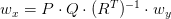
We use sp.linalg.lu_solve() to solve
 but
this expects to have arguments R^T = L*U where L has unit
diagonals, so we need to rescale R slightly.
but
this expects to have arguments R^T = L*U where L has unit
diagonals, so we need to rescale R slightly.Examples
>>> x = np.linspace(-1, 1, 102)[1:-1]
>>> wx_ = [2]
>>> n = 0
>>> while min(wx_) >= 0:
...     # Find maximum order with positive weights.
...     n += 1
...     y, wy = sp.special.orthogonal.p_roots(n)
...     wx = wx_
...     wx_ = get_weights_y(x, y, wy)
>>> n = n - 1
>>> print n
18
>>> np.allclose(np.dot(wx, x**16), 2./17)
True
>>> np.allclose(np.dot(wx, x**17), 0)
True
- mmf.math.integrate.integrate_1d.quadrature.integrate(f, a, b, abs_tol=None, rel_tol=None, points=None, singular_points=None, **kwargs)[source]
Return (res, err) where res is the integral of the function f(x) from a to b and err is an estimate of the absolute error.

Parameters : a, b : float
Limits of integration. These can be finite or infinite.
abs_tol, rel_tol : float
Desired tolerance goals.
points : list of floats
Points where the integrand is significant i.e. where does the integrand change behaviour. If there is a sharp feature, then it should be located by these points (the adaptive routine might otherwise miss it.). These points will be explicitly included in the integral so they should not be singular points.
singular_points : list of floats
List of singular points of the integrand. These will be excluded from the integral but approached with caution.
- mmf.math.integrate.integrate_1d.quadrature.quad(f, a, b, *varargin, **kwargs)[source]
An improved version of integrate.quad that does some argument checking and deals with points properly.
Return (ans, err).
Examples
>>> def f(x): return 1./x**2
>>> (ans, err) = quad(f, 1, np.inf, points=[])
>>> abs(ans - 1.0) < err
True
>>> (ans, err) = quad(f, 1, np.inf, points=[3.0, 2.0])
>>> abs(ans - 1.0) < err
True
- mmf.math.integrate.integrate_1d.quadrature.mquad(f, a, b, abs_tol=1e-12, verbosity=0, fa=None, fb=None, save_fx=False, res_dict=None, max_fcnt=10000, min_step_size=None, norm=<function <lambda> at 0xca6b1f0>, points=[])
Return (res, err) where res is the numerically evaluated integral using adaptive Simpson quadrature.
mquad tries to approximate the integral of function f from a to b to within an error of abs_tol using recursive adaptive Simpson quadrature. mquad allows the function y = f(x) to be array-valued. In the matrix valued case, the infinity norm of the matrix is used as it’s “absolute value”.
Parameters : f : function
Possibly array valued function to integrate. If this emits a NaN, then an AssertionError is raised to allow the user to optimize this check away (as it exists in the core of the loops)
a, b : float
Integration range (a, b)
fa, fb : float
f(a) and f(b) respectively (if already computed)
abs_tol : float
Approximate absolute tolerance on integral
verbosity : int
Display info if greater than zero. Shows the values of [fcnt a b-a Q] during the iteration.
save_fx : bool
If True, then save the abscissa and function values in res_dict.
res_dict : dict
Details are stored here. Pass a dictionary to access these. The dictionary will be modified.
max_fcnt : int
Maximum number of function evaluations.
min_step_size : float
Smallest step size limiting termination
norm : function
Function to compute the norm of the values of f(x). This allows the use to use matrices, vectors, etc. This norm is used to determine convergence.
points : list of floats
List of special points. The integral will be subdivided into these regions.
Notes
The basic idea here is to use a nested quadrature rule to assess the value of the integrand over a given integral, and then subdivide if tolerances are not met.
Based on “adaptsim” by Walter Gander. Ref: W. Gander and W. Gautschi, “Adaptive Quadrature Revisited”, 1998. http://www.inf.ethz.ch/personal/gander
Examples
Orthogonality of planewaves on [0, 2pi]
>>> def f(x):
...     v = np.exp(1j*np.array([[1.0, 2.0, 3.0]])*x)
...     return v.T.conj()*v/2.0/np.pi
>>> ans = mquad(f, 0, 2*np.pi)
>>> abs(ans - np.eye(ans.shape[0])).max() < _abs_tol
True
>>> res_dict = {}
>>> def f(x): return x**2
>>> ans = mquad(f, -2, 1, res_dict=res_dict, save_fx=True)
>>> abs(ans - 3.0) < _abs_tol
True
>>> x = np.array([xy[0] for xy in res_dict['xy']])
>>> y = np.array([xy[1] for xy in res_dict['xy']])
>>> abs(y - f(x)).max()
0.0
Handling singularities.
>>> def f(x): return 1.0/np.sqrt(x) + 1.0/np.sqrt(1.0-x)
>>> abs(mquad(f, 0, 1, abs_tol=1e-8) - 4.0) < 2e-7
True
Handling discontinuities.
>>> def f(x):
...     if x < 0:
...         return 0.0
...     else:
...         return 1.0
>>> abs(mquad(f, -2.0, 1.0) - 1.0) < 1e-10
True
>>> def f(x): return 1./x
>>> mquad(f, 1, np.inf)
Traceback (most recent call last):
    ...
ValueError: Infinite endpoints not supported.
- mmf.math.integrate.integrate_1d.quadrature.h_roots(n)[source]
Return the abscissa and weights for the Gaussian quadrature of order n in the Hermite polynomials.
Notes
We use the scipy routines for the roots, but our own custom formula for the weights because the scipy routine screws up these for large n.