mmf.fit.lsq
| leastsq(f, p0, x, y[, dy, df, scale_cov, ...]) | Return (p, dp, Q, cov) (or (p, dp, Q, cov, F) if df is |
| lsq(X, y[, dy]) | Return (a, cov, Q, residuals) for a least |
| lsqf(f, x, y, dy[, scale_cov, return_residuals]) | Return (a, cov, Q, F) or (a, cov, Q, F, residuals, chi2r) for a |
| lsqm(model, x, y, dy[, active]) | Perform a least squares fit using the functions defined in the |
| Delta(nu, sigma) | Return  required to estimate the errors for required to estimate the errors for  |
Least squares fitting with error estimates.
Linear Least Squares
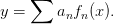
The simplest least-squares is the linear least squares approach which
involves fitting the coefficients  in an expansion of the form:
To view this as a linear algebra problem, define the matrix
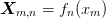
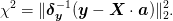
One can then write the problem as a standard least-squares problem of
minimizing the  fitness measure over the vector of parameters
 :
:
Error Estimates
Warning
The error estimates discussed here are only valid under the strict
assumption that the errors in the input data are normally distributed. In
this case – and when the model is linear over the region of variation –
then the covariance matrix  may be used to provide confidence estimates as
discussed below.
may be used to provide confidence estimates as
discussed below.
For a detailed discussion, please see [PTVF:2007] where they discuss
that, if you have non-normal errors, then you may still minimize the
to fit your parameters, and use the covariance matrix  to determine
the confidence contours. You may not estimate which confidence interval
the contours correspond to. To get this estimate, you must perform a Monte
Carlo simulation using the proper distribution function.
to determine
the confidence contours. You may not estimate which confidence interval
the contours correspond to. To get this estimate, you must perform a Monte
Carlo simulation using the proper distribution function.
The following discussion assumes that the input data has normally distributed errors.
Single Parameter Confidence Interval
When considering a single parameter on its own, the error returned represents
the  confidence interval (for normally distributed data) for that
parameter assuming that the additional parameters are chosen to minimize
. We provide two types of error and covariance estimates here depending
on the value of the scale_cov argument:
confidence interval (for normally distributed data) for that
parameter assuming that the additional parameters are chosen to minimize
. We provide two types of error and covariance estimates here depending
on the value of the scale_cov argument:
If scale_cov = False, then the error estimates describe the standard deviation of the distribution of the fitted parameters from a set of data with uncorrelated normal errors with the prescribed standard deviations dy. If the model is poor, or the errors are underestimated (very low quality of fit Q) , then this will give very small error (unreasonable) estimates for the parameters.
If scale_cov = True, then the covariance matrix is scaled by the reduced chi squared
 where
where  is the number of degrees of freedom (
 data points and
  parameters). This is equivalent to the previous case if
 , and so can be thought of as scaling the
error estimates dy to make the model fit. In essence, this
provides a much more reasonable estimate of the parameters
as a curve fitting problem, but will not have the proper
interpretation as in the prior case. This is what the scipy
documentation means when it states: “This matrix must be multiplied by the
residual standard deviation to get the covariance of the parameter
estimates” in the documentation of scipy.optimize.leastsq().
, and so can be thought of as scaling the
error estimates dy to make the model fit. In essence, this
provides a much more reasonable estimate of the parameters
as a curve fitting problem, but will not have the proper
interpretation as in the prior case. This is what the scipy
documentation means when it states: “This matrix must be multiplied by the
residual standard deviation to get the covariance of the parameter
estimates” in the documentation of scipy.optimize.leastsq().Note
One can estimate the scale_cov = True errors after the fact by simply scaling them by simply multiplying the covariance matrix by the reduced chi-squared
 . Likewise, the errors
can be scaled by
. Likewise, the errors
can be scaled by  .
.
In short, if the error estimates dy are trusted, then do not scale the covariance matrix, and take the quality of the fit Q seriously and rejecting the parameter estimates if it is too small. On the other hand, if the errors are not known, or one is imply trying to visually fit the data, then one should use the scaled covariance matrix.
If you need different confidence bands, then note that the error is related to the diagonal of the covariance matrix via:
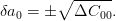
One can compute for the appropriate confidence level using
Delta(). Note that the argument denotes not how many parameters are
in the model, but should be thought of as the dimensionality of the confidence
ellipse. To estimate the error for a single parameter  (even if the
model has multiple parameters) with the standard (
(even if the
model has multiple parameters) with the standard ( ) confidence
interval,
) confidence
interval,  :
:
>>> Delta(nu=1.0,sigma=1.0)
1.0
Thus, you can simply multiply the error by  to find
the different confidence interval.
to find
the different confidence interval.
Multiple Parameter Confidence Intervals
The previous characterization of errors – and that returned in the parameter
error estimates – is valid when each parameter is considered independently
under the assumption that the other parameters are adjusted to minimize
. It is in general not valid when considering a group of parameters.
Instead, the confidence region of multiple parameters is in general described by
an ellipsoid described by the following procedure (see [PTVF:2007]):
Determine
such that  where
where  for one standard deviation,
  for two
standard deviations etc. Here is the number of parameters you
simultaneously want to describe (i.e. the dimension of the ellipsoid, not the
total number of parameters in the model).
for two
standard deviations etc. Here is the number of parameters you
simultaneously want to describe (i.e. the dimension of the ellipsoid, not the
total number of parameters in the model).The confidence ellipse is:
where
 is the block of the total covariance matrix
containing the corresponding parameters of interest, and
is the block of the total covariance matrix
containing the corresponding parameters of interest, and
 is the vector of the errors in those
parameters. This analysis assumes that the other parameters are
adjusted to minimize as these chosen parameters are
varied and as a result, is slightly smaller than the extremal
bounds of the confidence ellipse.
is the vector of the errors in those
parameters. This analysis assumes that the other parameters are
adjusted to minimize as these chosen parameters are
varied and as a result, is slightly smaller than the extremal
bounds of the confidence ellipse.
We present the result of this here in terms of a non-linear least
squares formula. Suppose that  , then within the
error ellipse we have
, then within the
error ellipse we have

If we diagonalize  where
where
 is diagonal, then we can write the maximum value of
  as
as
Thus, we simply find the maximum and minimum components of the vector
 and we have the range of
errors in . For the linear model
and we have the range of
errors in . For the linear model  .
.
Example
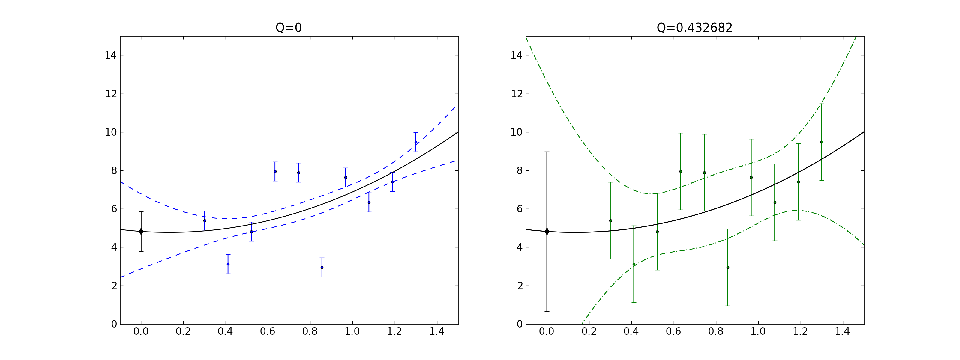
Here we demonstrate this with a polynomial fit with data sampled with a Gaussian distribution. We generate the data with a fixed standard deviation, but first underestimate the errors. We then apply the scale_cov=True and show that this is consistent with a proper error estimate.
plt.figure(figsize=[16,6])
plt.subplot(121)

import mmf.fit.lsq
np.random.seed(0)
fs = [lambda x:1, lambda x:x, lambda x:x*x]
def f(x, p): return fs[0](x)*p[0] + fs[1](x)*p[1] + fs[2](x)*p[2]
x = np.linspace(0.3, 1.3, 10); p0 = [1, 2, 3]; y0 = f(x, p0)
X = np.linspace(-0.1, 1.5, 100)

dy0 = 2.0                 # Large scatter in points
y = y0 + np.random.normal(0, dy0, len(y0))
dy = 0.5                  # Underestimate of errors

plt.subplot(121)
(p, cov, Q, F) = mmf.fit.lsq.lsqf(fs, x, y, dy=dy, scale_cov=False)

plt.errorbar(x, y, 0*y + dy, fmt='.b', ecolor='b')
plt.errorbar(0, p[0], np.sqrt(cov[0,0]), fmt='dk')
plt.plot(X, F(X, a=p)[0], '-k',
         X, F(X, a=p)[0] + F(X, a=p)[1], '--b',
         X, F(X, a=p)[0] - F(X, a=p)[1], '--b')
plt.title("Q=%g" % Q)
plt.axis((-0.1,1.5,0,15))

plt.subplot(122)
(p, cov, Q, F) = mmf.fit.lsq.lsqf(fs, x, y, dy=dy, scale_cov=True)

plt.errorbar(x, y, 0*y + dy0, fmt='.g', ecolor='g')
plt.errorbar(0, p[0], np.sqrt(cov[0,0]), fmt='dk')
plt.plot(X, F(X, a=p)[0], '-k',
         X, F(X, a=p)[0] + F(X, a=p)[1], ':g',
         X, F(X, a=p)[0] - F(X, a=p)[1], ':g')

(p, cov, Q, F) = mmf.fit.lsq.lsqf(fs, x, y, dy=dy0, scale_cov=False)
plt.errorbar(0, p[0], np.sqrt(cov[0,0]), fmt='dk')
plt.plot(X, F(X, a=p)[0], '-k',
         X, F(X, a=p)[0] + F(X, a=p)[1], '--g',
         X, F(X, a=p)[0] - F(X, a=p)[1], '--g')
plt.title("Q=%g" % Q)

plt.axis((-0.1,1.5,0,15))
(Source code, png, hires.png, pdf)
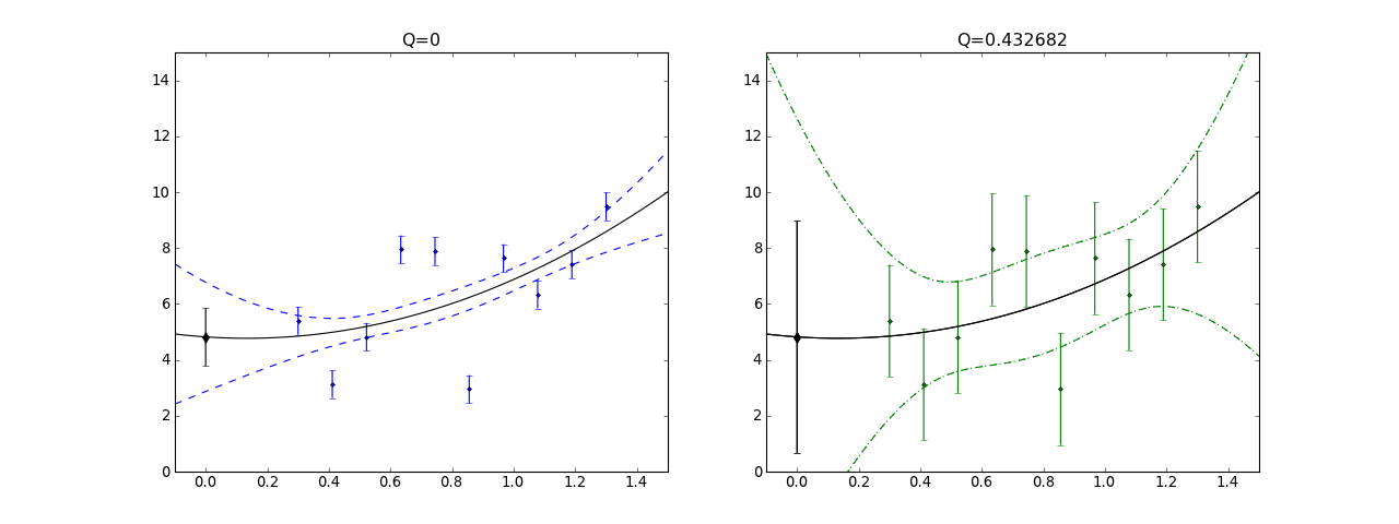
As an example, here is a plot of some data scattered with a standard deviation of 2 but fit with underestimated errors of 0.5 (left). The quality of this fit is extremely poor (Q=0) and the error bounds (blue dashed curves) are correspondingly underestimated. This is the type of fluctuation that the fitted curve would exhibit if the data fluctuated with the smaller standard deviation, but does not describe the scatter in the data. If the error bars are trusted here and the errors are normally distributed etc. then one would have to conclude that the model is not very good.
On the right we consider the same fit, but with scale_cov = True (green dotted curves) which much better captures the visual scatter of the data. In fact, this agrees with the error bounds (green dotted curves) that are obtained by setting the appropriate standard deviation dy = 2 (green error bars) with scale_cov = False. In this case the quality of the fit Q = 0.4 is good and the error bound agree well “visually” with the scatter in the data. This shows how – if one has normally distributed errors of the same size – one can use scale_cov=True to estimate the errors.
Finally, since this is a polynomial model, one might think that the error in the
intercept would be simply the error in the parameter  (shown as a black
error bar with a diamond at
(shown as a black
error bar with a diamond at  ). This is the confidence interval
for the single parameter when all other parameters are adjusted to
minimize the . This corresponds to
). This is the confidence interval
for the single parameter when all other parameters are adjusted to
minimize the . This corresponds to 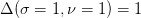 . The
error band shown in the previous plot corresponds to the joint error keeping all
three parameters fixed
. The
error band shown in the previous plot corresponds to the joint error keeping all
three parameters fixed 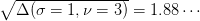 which is the
larger ellipse shown below. This is a projection of the “joint”
distribution ellipsoid for all three parameters.
which is the
larger ellipse shown below. This is a projection of the “joint”
distribution ellipsoid for all three parameters.
plt.figure(figsize=[16,6])

import mmf.fit.lsq
np.random.seed(0)
fs = [lambda x:1, lambda x:x, lambda x:x*x]
def f(x, p): return fs[0](x)*p[0] + fs[1](x)*p[1] + fs[2](x)*p[2]
x = np.linspace(0.3, 1.3, 10); p0 = [1, 2, 3]; y0 = f(x, p0)
X = np.linspace(-0.1, 1.5, 100)

dy = 2.0
y = y0 + np.random.normal(0, dy, len(y0))

(p, cov, Q, F) = mmf.fit.lsq.lsqf(fs, x, y, dy=dy, scale_cov=False)

# Generate ellipses for 2-parameters a_0 and a_1
def error_band(Cproj, sigma=1.0, nu=1.0):
    u, d, vt = np.linalg.svd(Cproj)

    Delta = mmf.fit.lsq.Delta(sigma=sigma, nu=nu)
    theta = np.linspace(0, 2.0*np.pi, 100)
    dx = np.sqrt(Delta)*np.exp(1j*theta)
    dp = np.dot(np.dot(u*np.sqrt(d),vt), [dx.real, dx.imag])
    assert np.allclose(Delta,
                       (np.dot(dp.T, np.linalg.inv(Cproj))*dp.T).sum(axis=1))

    return dp

plt.subplot(121)
C01 = cov[:2,:2]
ls = ['k-', 'g:', 'b--']
for _l, _nu in enumerate([1,2,3]):
    dp = error_band(C01, nu=_nu)
    plt.plot(p[1] + dp[1], p[0] + dp[0], ls[_l])
    Delta = mmf.fit.lsq.Delta(sigma=1.0, nu=_nu)
    plt.axhline(p[0] + np.sqrt(Delta*cov[0,0]), c=ls[_l][0], ls=ls[_l][1])
    plt.axhline(p[0] - np.sqrt(Delta*cov[0,0]), c=ls[_l][0], ls=ls[_l][1])

plt.xlabel("a_1")
plt.ylabel("a_0")

plt.subplot(122)
C02 = cov[[0,2],:][:,[0,2]]
for _l, _nu in enumerate([1,2,3]):
    dp = error_band(C02, nu=_nu)
    plt.plot(p[2] + dp[1], p[0] + dp[0], ls[_l])
    Delta = mmf.fit.lsq.Delta(sigma=1.0, nu=_nu)
    plt.axhline(p[0] + np.sqrt(Delta*cov[0,0]), c=ls[_l][0], ls=ls[_l][1])
    plt.axhline(p[0] - np.sqrt(Delta*cov[0,0]), c=ls[_l][0], ls=ls[_l][1])

plt.xlabel("a_2")
plt.ylabel("a_0")
(Source code, png, hires.png, pdf)
The functions defined here perform linear least-squares fitting and non-linear fitting, using scipy.optimize.leastsq().
Polynomial Fit Revisited
References
| [PTVF:2007] | (1, 2, 3, 4, 5) William H. Press, Saul A. Teukolsky, William T. Vetterling, and Brian P. Flannery, “Numerical Recipes: The Art of Scientific Computing”, Cambridge University Press, (2007) |
- mmf.fit.lsq.leastsq(f, p0, x, y, dy=None, df=None, scale_cov=False, epsfcn=0.0, factor=100, ftol=1e-08, diag=None)[source]
Return (p, dp, Q, cov) (or (p, dp, Q, cov, F) if df is provided) for a a least-square fit of the function y = f(x, p) for the parameters p.
Parameters : f : function
This should be a vectorized function f(x, p). A common example for polynomial fitting is:
def f(x, p):
    return np.polyval(p, x)
df : function, (optional)
This should return the derivatives of f with respect to the parameters as a column vector (broadcast as x[None, :] and p[:,None]), for example, for polynomial fitting:
def df(x, p):
    return x**np.arange(len(p))[::-1,None]
p0 : array
Initial guess for parameters.
x, y : array
This is the data
dy : array, (optional)
The errors. These should be the standard deviations for the values y. (The whole analysis is predicated on the assumption of Gaussian errors.)
scale_cov : bool, (optional)
If this is True, then the covariance matrix and error estimates will be scaled by chi/sqrt(nu) where nu = len(x) - len(p) is the number of degrees of freedom. This scaling allows one to extract parameter estimates even if the errors dy are not properly estimated.
Note
We do not use Bessel’s correction here (which would count the number of degrees of freedom as nu = len(x) - len(p) -1). This might lead to a slight bias in the error estimates but allows the code to work in plausible cases such as fitting two-points with one parameter. We follow [PTVF:2007] here, not Wikipedia for example.
Returns : p : array
Parameter estimates (mean values).
dp : array
Estimate of the errors in parameters assuming that they are independent. Note that the actual 1-sigma confidence region for the parameters is the ellipsoid

The meaning of these errors are that if a set of data is generated with uncorrelated normally distributed errors in y with standard deviation dy about mean values f(x, p), then the estimates for the parameters p resulting from the fits will be approximately normally distributed with standard deviation dp.
cov : array
Two-dimensional covariance matrix
. This defines the
1-sigma confidence interval if the errors are normally
distributed.Q : float
Quality of fit (should be between 0.01 and 0.1). If errors are not specified or are inaccurate, then this is meaningless.
Examples
We start with a linear example of polynomial fitting as discussed above:
>>> def f(x, p):
...     return np.polyval(p, x)
>>> def df(x, p):
...     return x**np.arange(len(p))[::-1,None]
Here are our parameters f = 1 + 2*x + 3*x**2 and some errors:
>>> p0 = [3, 2, 1]
>>> dp0 = [0.03, 0.02, 0.01]
Let’s generate some normally distributed data over an abscissa with some errors dy that we can estimate using standard error analysis:
>>> np.random.seed(1)
>>> x = np.linspace(0, 3, 50)
>>> dy = np.sqrt(((df(x, p0)*np.array(dp0)[:,None])**2).sum(axis=0))
>>> y = f(x, p0) + np.random.normal(0, dy, len(x))
Now we do the fit: we try with and without df to ensure that both are the same:
>>> p,dp,Q,cov = leastsq(f=f,p0=[0,0,0],x=x,y=y,dy=dy)
>>> p1,dp1,Q1,cov1,F = leastsq(f=f,p0=[0,0,0],x=x,y=y,dy=dy,df=df)
>>> (np.allclose([p, dp], [p1, dp1]), np.allclose(cov, cov1))
(True, True)
Providing the derivative allows us to reduce the number of function calls though. Now we generate a bunch of data and tabulate the fitted parameter values to see if the error estimates are reasonable:
>>> P_ = np.array([
...     leastsq(f=f, p0=p, x=x, dy=dy, df=df,
...             y = f(x, p0) + np.random.normal(0, dy))[0]
...     for n in xrange(100)])
>>> P_.mean(axis=0)
array([ 3.00..., 2.00..., 0.99...])
>>> P_.std(axis=0)
array([ 0.012...,  0.022...,  0.0058...])
This agrees with the previously calculated errors of the fit:
>>> dp
array([ 0.012...,  0.020...,  0.0058...])
Note
The precise meaning of this error estimate is to describe the standard deviation of the fitted parameter values give independent normally distributed errors in the data with standard deviation dy. These are not estimates of the distribution of the original parameters which would be determined directly from the errors in the data:
>>> np.sqrt(np.dot(np.linalg.pinv((df(x, p0).T**2)), dy**2))
array([ 0.03,  0.02,  0.01])
This relationship between dy and the distribution of the original parameters has nothing to do with the fit. Were we to provide more data for the fit, the error in the parameters dp would decrease: we determining the mean of the parameter distribution more and more precisely.
We also consider the extrapolation error using the model with the fitted parameters
>>> x0 = 5.0                # Extrapolate to here
>>> y0_ = np.array([
...     f(x0, leastsq(f=f, p0=p, x=x, dy=dy, df=df,
...                   y = f(x, p0) + np.random.normal(0, dy))[0])
...     for n in xrange(200)])
>>> y0_.mean(), y0_.std()
(86.00..., 0.227...)
>>> F(x0)
(86.18..., 0.220...)
This agrees with the previously calculated errors of the fit:
>>> dp
array([ 0.012...,  0.020...,  0.0058...])
Now we consider a non-linear model:
First we generate some data, then we fit and extract the parameters
>>> import numpy as np
>>> from numpy import linspace, array, mean, std, ones, sqrt
>>> from numpy.random import normal as rand
>>> np.random.seed(1)
>>> def f(x, m, mu, Delta):
...    return sqrt((x**2/2/m-mu)**2+Delta**2)
>>> m, dm = 2.0, 0.01
>>> mu, dmu = 2.0, 0.02
>>> Delta, dDelta = 2.0, 0.03
>>> x = linspace(0, 3, 50)
>>> def get_y_dy(x, N=1000):
...     ys = [f(x0, rand(m,dm), rand(mu,dmu), rand(Delta,dDelta)) for
...           x0 in x*ones(N)]
...     y = ys[0]
...     dy = std(ys)
...     return (y,dy)
>>> y_dy = [get_y_dy(x0) for x0 in x]
>>> y = [ydy[0] for ydy in y_dy]
>>> dy = [ydy[1] for ydy in y_dy]
>>> #from pylab import errorbar,ion,clf
>>> #ion();clf()
>>> #errorbar(p,y,dy);
>>> #import pdb;pdb.set_trace()
>>> def fn(p, params):
...     m, mu, Delta = params
...     return f(p,m,mu,Delta)
>>> p, err, Q, cov = leastsq(fn, [m, mu, Delta], x, y, dy)
Is the fit is good?
>>> Q
0.6...
Yes. This is a Gaussian model and so the fit should be good. In general, if the Gaussian approximation is not perfect, then Q may be lower. Values of 0.001 may still be acceptable. We check that the error estimates are also reasonable:
>>> abs(p - array([m, mu, Delta]))/err
array([ 1.3...,  1.6..., 1.6...])
A brief note about how the errors and covariances scale. If we scale the errors dy by a common factor s, then the fit p remains unchanged while the error-estimates scale by s and the covariance matrix scales by s**2:
>>> s = 0.5
>>> dy1 = s*np.array(dy)
>>> p1, err1, Q1, cov1 = leastsq(fn, [m, mu, Delta], x, y, dy1)
>>> np.allclose(p, p1)
True
>>> np.allclose(err1, s*err)
True
>>> np.allclose(cov1, s**2*cov)
True
Note that the Q value is horrible though because we have made the errors too small.
>>> Q1
1...e-16
The argument scale_cov scales the errors in this way so that the reduced
 would be one, and uses this to estimate the
errors.
would be one, and uses this to estimate the
errors.>>> chi2 = (((fn(x, p1) - y)/dy1)**2).sum() >>> chi2_r = chi2/(len(x) - len(p1)) >>> s1 = np.sqrt(chi2_r) >>> p2, err2, Q2, cov2 = leastsq(fn, [m, mu, Delta], x, y, dy1, ... scale_cov=True) >>> np.allclose(err2, err1*s1) True
- mmf.fit.lsq.lsq(X, y, dy=None)[source]
Return (a, cov, Q, residuals) for a least squares fit of the linear least squares problem
Parameters : X : 2d array X x Na
Abscissa. Least square problem is norm(dot(X, a) - y).
y : (N x 1) array of floats
Data values.
dy : (N x 1) array of floats, optional
Errors in data (assumed to be normally distributed). Assumed to be 1 if not provided.
Returns : a : vector
Vector of parameters estimates
cov : matrix
Covariance matrix
Q : float
Estimate of the goodness of the fit. (Q should be between 0.001 and 0.1. Larger values indicate that the errors have been over-estimated. Smaller values mean that the model is bad, or the errors have been underestimates, or the errors are not normally distributed.
References
See [PTVF:2007].
- mmf.fit.lsq.lsqf(f, x, y, dy, scale_cov=False, return_residuals=False)[source]
Return (a, cov, Q, F) or (a, cov, Q, F, residuals, chi2r) for a least squares fit of the data (x, y) to the function:
y = a[0]*f[0](x) + a[1]*f[1](x) + ...
Parameters : f : 1d array of Na functions
x : 1d array of N parameters
Abscissa
y : 1d array of N floats
Data values
dy : 1d array of N floats
Errors in data (assumed to be normally distributed).
scale_cov : bool, (optional)
If this is True, then the covariance matrix and error estimates will be scaled by chi/sqrt(nu) where nu = len(x) - len(p) is the number of degrees of freedom. This scaling allows one to extract parameter estimates even if the errors dy are not properly estimated.
return_residuals : bool
If True, then data residuals will be returned.
Returns : a : vector
Vector of parameters estimates
cov : matrix
Covariance matrix
Q : float
Estimate of the goodness of the fit. (Q should be between 0.001 and 0.1. Larger values indicate that the errors have been over-estimated. Smaller values mean that the model is bad, or the errors have been underestimates, or the errors are not normally distributed.
F : function
This function takes abscissa x -> (y,dy) where y = f(x) is the best fit and dy is the estimated error. The error estimate uses the full covariance matrix.
residuals : Residuals if return_residuals is True.
chi2r : Reduced chi square if return_residuals is True.
References
See [PTVF:2007].
Examples
Generate a bunch of points on the parabola y = x**2-2*x+1 with errors and fit them.
>>> scipy.random.seed(0)
>>> N = 100
>>> f = [lambda x:1.0,lambda x:x,lambda x:x**2]
>>> a0 = [1.0,-2.0,1.0]
>>> Na = len(a0)
>>> def F(x,a=a0,f=f):
...     y = np.zeros(len(x),float)
...     for n in xrange(len(a)):
...         y += a[n]*f[n](x)
...     return y
>>> x = scipy.random.uniform(-3,3,N)
>>> dy = scipy.random.uniform(0,0.1,N)
>>> y = scipy.random.normal(F(x, a=a0),dy)
>>> a, cov, Q, F = lsqf(f,x,y,dy)
>>> assert Q < 0.9 and 0.1 < Q, "Q value not good for data! Q=%f" % Q
>>> #from pylab import *;ion();clf()
>>> #errorbar(x,y-F(x, a=a)[0],dy,fmt='.')
>>> #X = np.linspace(-3,3,1000)
>>> #Y,dY = F(X, a=a)
>>> #plot(X,dY,X,-dY)
- mmf.fit.lsq.lsqm(model, x, y, dy, active=None)[source]
Perform a least squares fit using the functions defined in the model dictionary and return a dictionary of results as (value,err) pairs.
- mmf.fit.lsq.Delta(nu, sigma)[source]
Return
required to estimate the errors for
parameters within a confidence interval of  standard
deviations.
standard
deviations.
where
 is the desired confidence from the normal
distribution. I.e. for
is the desired confidence from the normal
distribution. I.e. for  ,
,  for
for
 etc.
etc.Examples
>>> Delta(1, 1)
1.0
>>> Delta(1, 2)
3.9999...
>>> Delta(2, 1)
2.295...
>>> Delta(4, 2)
9.715...