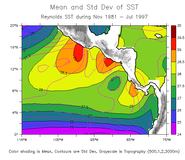
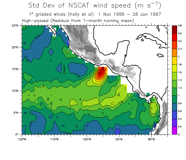
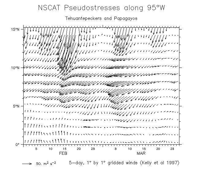
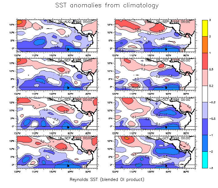
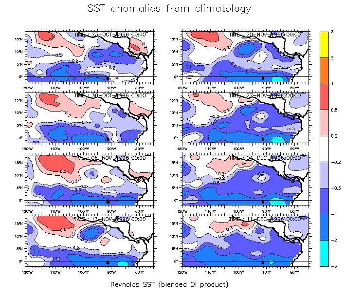
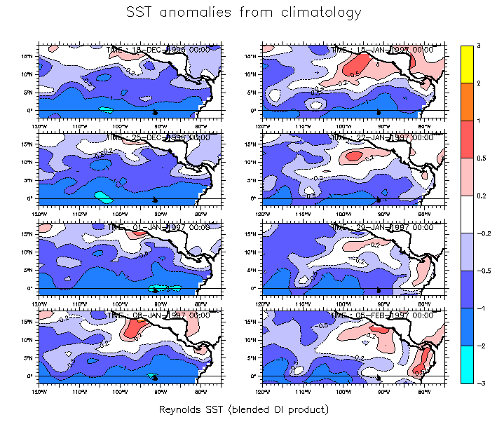
The dramatic effects on the Pacific of the strong winds that blow through the mountain gaps in Central America have been known for more than 35 years. Strong down-gradient winds occur through the three passes 10-12 times each boreal winter. Wind speeds can be as large as 20 m/s, and the events typically last for 5-7 days. These winds are due to winter synoptic high pressure events over the Great Plains, extending south over the Gulf of Mexico. Probably the most climatologically important aspect of this phenomenon is the rapid cooling that occurs in boreal fall when strong winds blow on this region with its very shallow summer thermocline. However, the winds also generate long-lived anticyclonic eddies that have been explained as the result of offshore winds exciting an initially symmetric pair of eddies, but immediately destroying the cyclonic (upwelling) one through entrainment under strong winds (McCreary et al, 1989, JMR p81). The purpose of this talk is to suggest that other processes may well contribute to the process of eddy formation; in particular there seems to be a connection to the reflection of intraseasonal equatorial Kelvin waves.
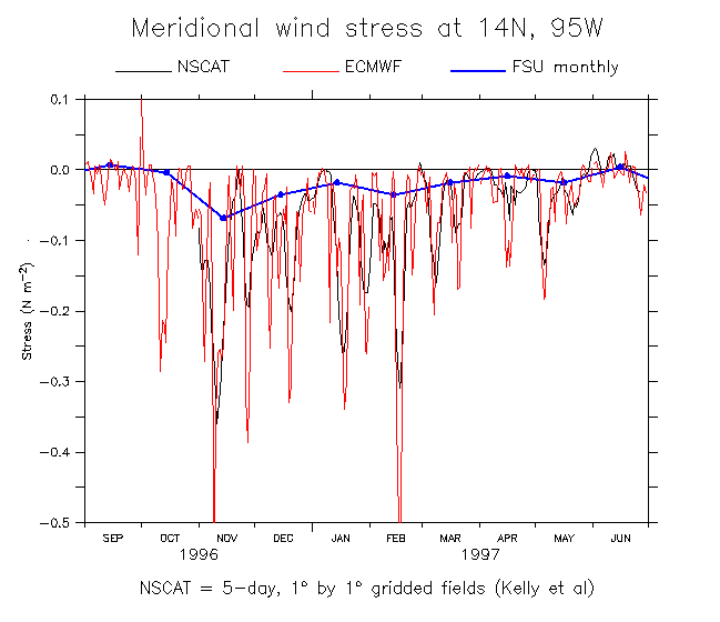
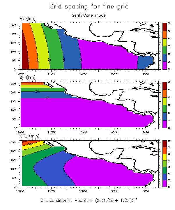
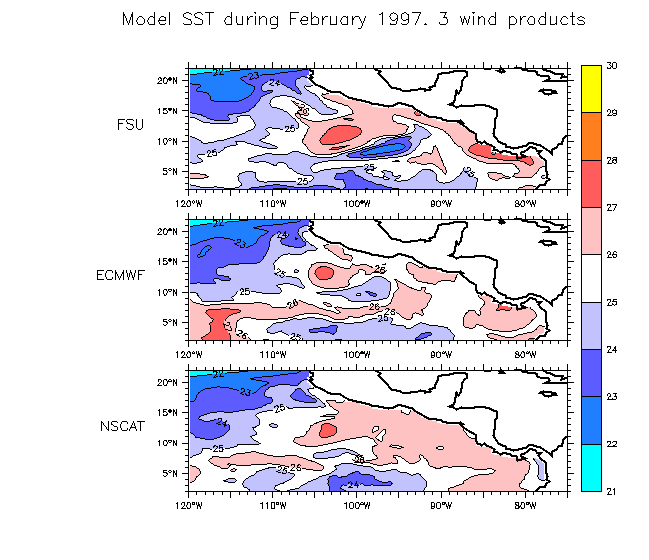
The Gent/Cane OGCM was forced with the three wind products. This is a high time and space resolution version of the model (20 minute timestep, 20 km grid spacing in the Central American region (see the grid spacing for the fine-grid runs)). The model was first spun up with 3 years of the FSU 1961-91 climatological winds. For the ECMWF and FSU runs, these winds were imposed beginning 1 January 1996 (model year 4). The NSCAT run was started from the results of the ECMWF run on 1 November 1996. All the runs were carried through the NSCAT period (to 26 June 1997). Results discussed below are from these runs.
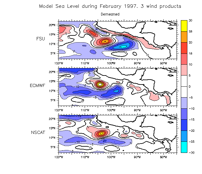
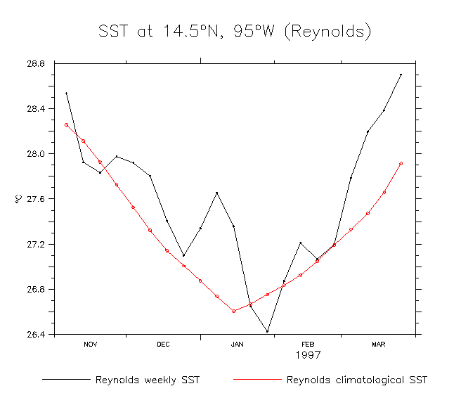
Based on the differences among the wind products shown in Fig. 4, we expected to see substantial differences among the model solutions. Surprisingly, this was not the case. Figs. 5 and 6 show the model SST and sea level during February 1997, for the three wind products.
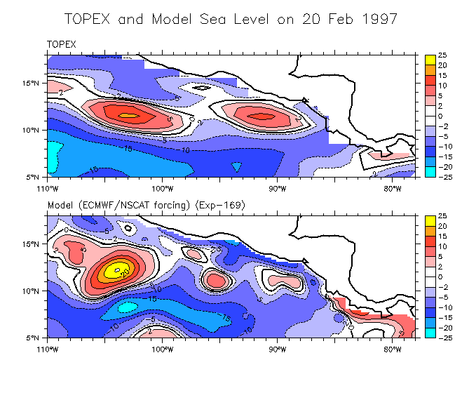
Comparing the observed and model fields in a time-longitude plot shows that the model representation of the time evolution is fairly realistic:
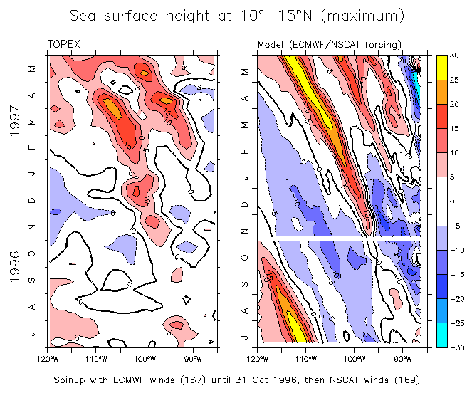
This raises the question of what generated these eddies. It is usually thought that the mountain-gap winds produce the eddies (through the process explained by McCreary et al, 1991). But then why were there more than 10 strong wind events but only 2 large and 2 small eddies during the winter of 1996-97? And why do the eddies seem to be traceable back to well before the wind events occurred?
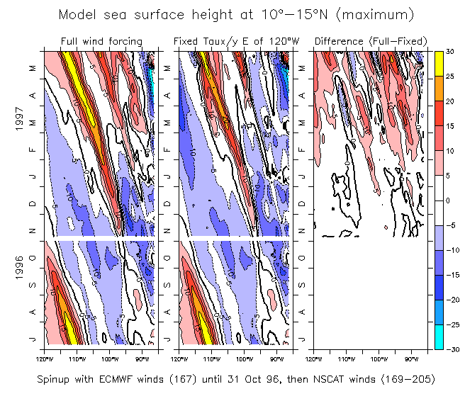
To further explore these questions, a model run was made in which the winds forcing the model east of 120°W were fixed to their 1 November 1996 values from that date onwards. Wind forcing variability continued as observed west of 120°W, but in the eastern Pacific it remained constant thereafter. Thus there were no mountain-gap winds forcing the model during boreal winter 1996-97. Fig. 9 compares the full model solution (same as the right panel of Fig. 8) with the fixed-wind solution, and the difference between the two..
Surprisingly, the solution without any mountain-gap winds still retains most of the same eddies in recognizable form, though with amplitude reduced by about a factor of two. Apparently the model eddies, at least, are not entirely generated by the mountain-gap winds. A second surprise is that the difference field is quite similar to the fixed wind solution. In a linear sense, one can think of the middle panel of Fig. 9 as representing the effect of the west Pacific winds, and the right panel as the effect of the east Pacific winds. Why should these be similar? Why should both elements of the wind field have a similar effect on the eastern ocean? A third surprise is that the eddies in both elements of the solution grow as the eddies move west.
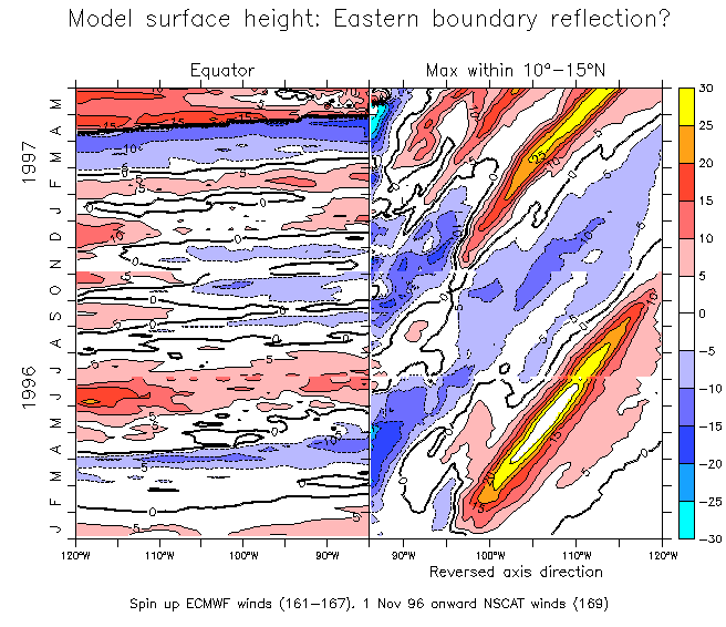
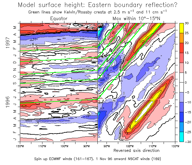
A possibility for surprise number one is suggested by Fig. 10, which shows that the three "Tehuantepec eddies" during boreal winter 1996-97 emanated from the boundary apparently as the reflection of equatorial Kelvin waves. The Rossby wave speed appears to be about 11 cm/s, which would imply that the long gravity wave speed c is about 2.2 m/s in this region. However, it is clear from the second of Figs. 10 (with overlaid crest lines), that the propagation speed is not perfectly constant, but appears to increase slightly to the west (consistent with the westward deepening of the thermocline?).
In addition, there is an ambiguity about the starting point of Rossby reflection, since these figures show the maximum sea level between 10° and 15°N, and due to the tilt of the coast the boundary longitude changes from about 85°W to 93°W in this range. Since the eddies appear at different latitudes (e.g. Fig. 7), it is not clear where the signal leaves the boundary, and therefore estimating where the reflection crest lines should go in Figs. 10 is uncertain.
Nevertheless, the hypothesis suggested by Figs. 9 and 10 is that the reflected (high sea level) Kelvin waves are a necessary element for the generation of Tehuantepec eddies. This would explain why there were many more mountain-gap wind events than resulting eddies. Perhaps the anticyclonic relative vorticity of the high sea level reflecting Kelvin waves preconditions the ocean to spin up eddies more efficiently. This would also explain why the two elements of the solution shown in Fig. 9 have very similar phase. This might also help to explain why only anticyclonic eddies are observed (e.g. McCreary et al 1991).
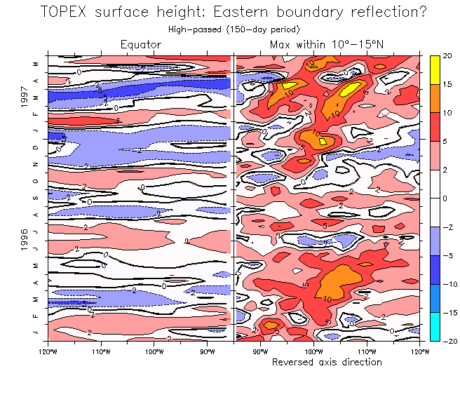
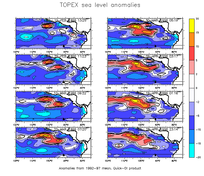
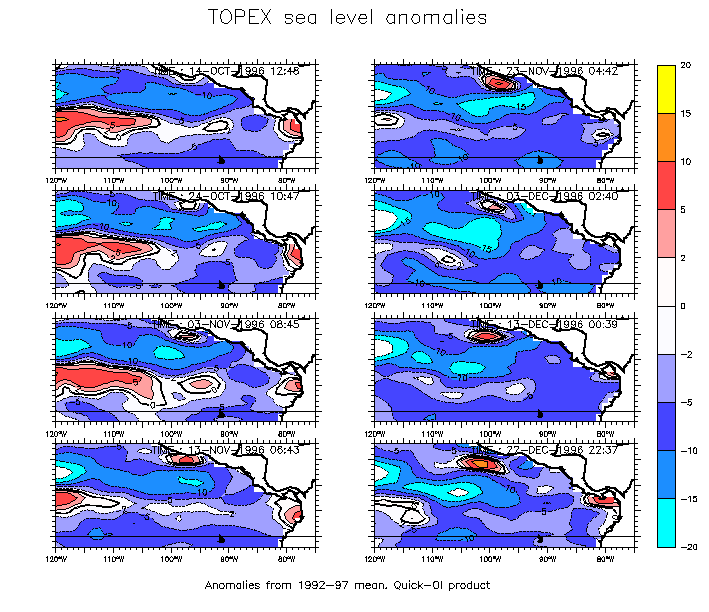
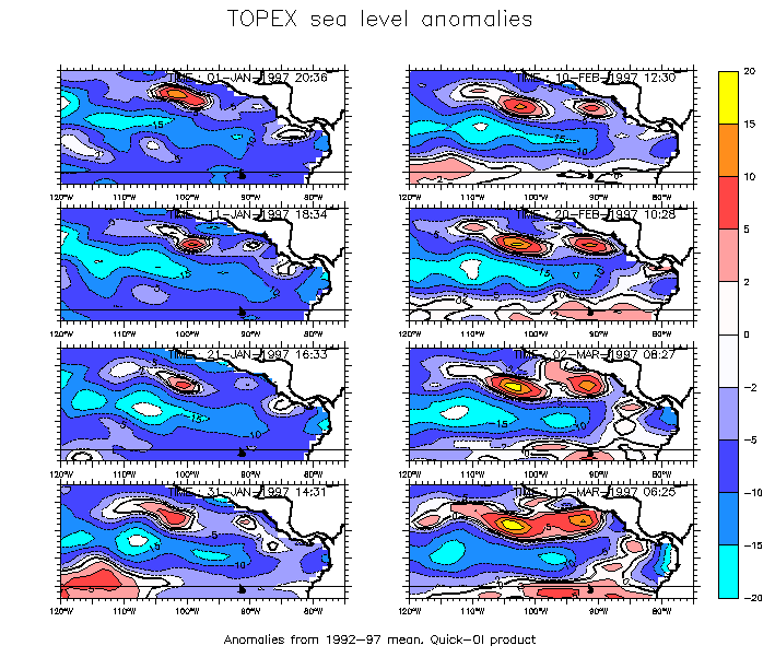
The corresponding picture from the TOPEX altimeter is somewhat less obvious, especially since (as also seen in Figs. 7 and 8 above) the model has two distinct eddies at 95°W-88°W where the altimeter shows one large eddy:
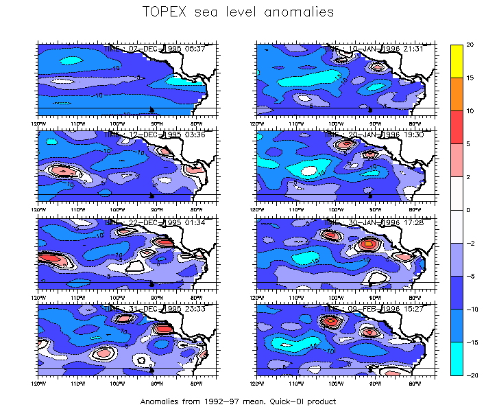
10-day maps of TOPEX sea level anomalies in the region SW of Central America
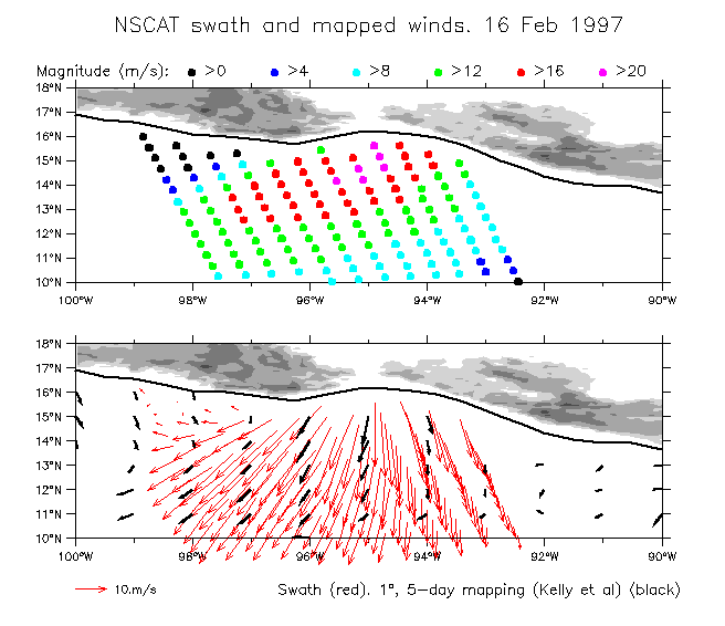
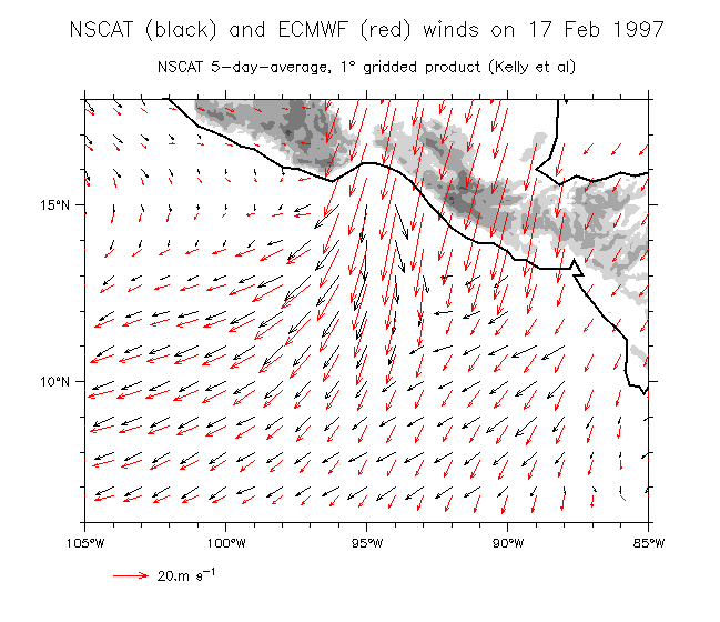
Winds
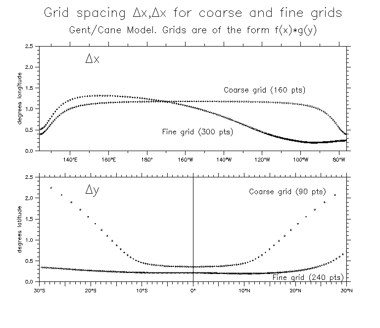
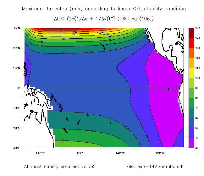
To make these runs resolving the Pecker eddies, I ran the model with a roughly 20km grid spacing in the eastern region. The CFL condition then required a 30-minute timestep. So I spent a lot of time waiting for the computer to grind through, and filled up a lot of disk space, too. Here's documentation of the grid: