Orthogonal Collocation Method for a Chemical Reactor with Radial Dispersion
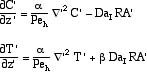
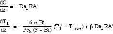
The problem is for flow and reaction as a fluid moves down a packed bed, filled with catalyst. The equations are derived elsewhere (link). Here we repeat them in nondimensional form.
![]()
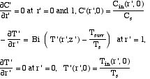
The boundary and initial conditions are
The orthogonal collocation method is applied by evaluating the differential equations at the collocation points and setting this residual to zero. We use symmetric polynomials since the solution is the same on either side of the centerline.

The boundary and initial conditions are

The conditions at the centerline are satisfied automatically with the symmetric polynomials. It is convenient to solve the last two equations and substitute into the differential equations.

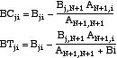
Alternatively, the differential equations can be written as
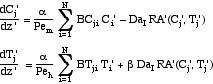
where
The Matlab code is available.
For the first approximation, the equations are
This approximation gives an insight to the physical situation. The equations take the same form as a lumped parameter model (link) of the same reactor, when radial gradients are not allowed.
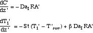
Here the Stanton number is
![]()
The two equations are the same provided
![]()
or when
![]()
The relative importance of the wall resistance is evident by computing the two terms in this equation. Comparing 1/hw to 1/U gives an idea of the fraction of the total heat transfer resistance that occurs at the wall. The equivalent comparison is
![]()
This ratio says that when Bi = 1, 75 % of the resistance is at the wall; when Bi = 10, only 23% of the resistance is at the wall; when Bi = 20, only 13% of the resistance is at the wall. When most of the resistance is at the wall, we expect small radial gradients. In that case the lumped parameter model or an orthogonal collocation approximation with N = 1 is sufficient. The orthogonal collocation
method provides a way to assess the accuracy of the lumped parameter model, since N can be increased and differences shown as the approximation to the partial differential equation improves.
The parameters for the first problem are
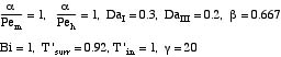
This case represents one with the majority of the heat transfer resistance at the wall. Solutions
for the radially-averaged concentration and temperature are shown in the figures.
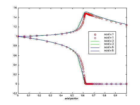
Clearly N = 1 is close, but N = 2 gives essentially the exact result. The corresponding radial profiles are shown in the next two figures.
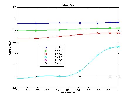
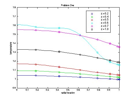
These figures confirm that fact that the radial profiles are almost flat, the only discrepancy being when the temperture rises sharply and the conversion becomes complete.
The parameters for the second problem are the same except for
![]()
This case represents one with the majority of the heat transfer resistance in the packed bed itself. Solutions for the radially-averaged concentration and temperature are shown in the figures.
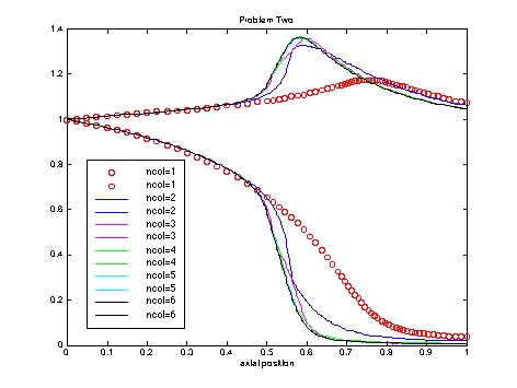
Clearly N = 1 is no good at all, N = 2 is still deficient, but N = 3 and higher gives a good result. The corresponding radial profiles are shown in the next two figures.
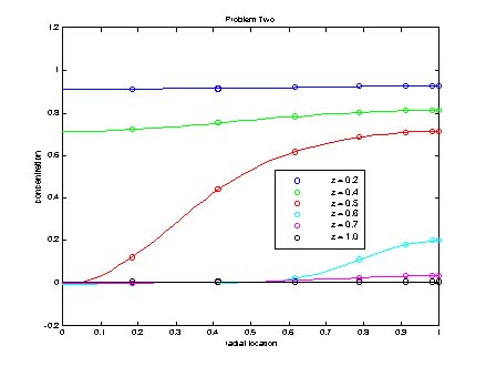
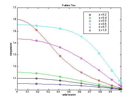
These figures confirm that fact that the radial profiles are more important when the Biot number is larger.
Take Home Message: When radial profiles are important, the orthogonal collocation method using only a few terms is an excellent method.