Orthogonal Collocation on Finite Elements for Axial Dispersion Problems
The orthogonal collocation method on finite elements is a useful method for problems of axial dispersion in reactors, especially when the solution has steep gradients. Here we apply the method to the case of a reactor with a second order chemical reaction, and then apply it to a nonisothermal problem (which is when steep gradients often occur).
Consider first the case of a reaction that is second order in concentration.
![]()
The orthogonal collocation on finite elements divides the domain, 0 x 1, into finite elements, and sets the residual to zero at the collocation points interior to the elements. The numbering system is shown in the figure.
![]()
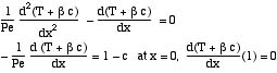
Then the equations become
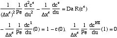
in each element. The orthogonal collocation method is applied at each collocation point interior to the element.
![]()
In addition, continuity of the function and first derivative between elements requires the condition
![]()
The function is continuous by virtue of assigning it only one value, regardless of whether it is the last point on one element or the first point on the next element. The continuity of first derivative is enforced using
![]()
at the points between elements. At the inlet the boundary condition is
![]()
and at the outlet the boundary condition is
![]()
Typically, the Newton Raphson method is used to solve nonlinear problems. The nonlinear reaction rate term is expended to give
![]()
The problem is solved using the general form
![]()
In this form, we need

The code is available.
First consider the case with a fixed Peclet number of 10 (a low value), and vary the
Damköhler number from 0.1 to 10. Typical solutions are shown in the figure.
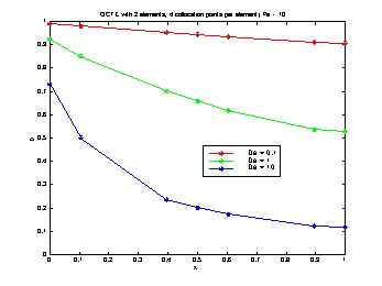
Figure 1. Axial Dispersion Model, Second-order Reaction
These results were generated by using 2 elements and 4 collocation points per element, and
are hardly changed when using more elements or collocation points; for small Damköhler numbers
they are accepted as accurate enough. For Da = 10, more points or elements are needed, and the
convergence is shown in Figure 2; 2 elements are not enough, but 4 are enough.
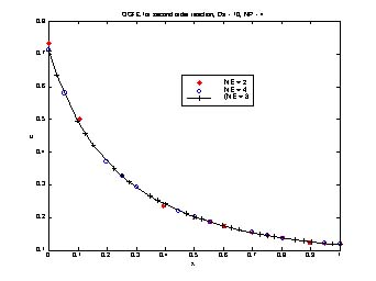
Figure 2. Convergence of Axial Dispersion Model, Pe = 10, Da = 10
Now vary the Peclet number, for the case of Da = 1. The solution for the highest Pe needs a few more points. Of course, all plots would be improved if we use the interpolation with polynomials rather than straight line interpolation.
Figure 3. Axial Dispersion Model, Second-order Reaction, High Peclet Numbers
Next consider the nonisothermal problem.
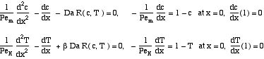
where the rate of reaction is taken as
![]()
Now, steep gradients can be formed because as the reaction proceeds, energy is given off (for an exothermic reaction), and the reaction proceeds even faster. This problem has the feature that, if the two Peclet numbers are the same, the two equations can be combined into one. Multiply the concentration equations by b and add to the temperature equations. The result is
The solution to this equation is
![]()
Thus, one can solve only the first equation for concentration, using the relation above to obtain the temperature from the concentration at any position.
When the Peclet numbers are different, one must solve both equations simultaneously. In either case, convergence can be difficult because of the strong temperature dependence in the reaction rate. The solutions obtained here using orthogonal collocation on finite elements were obtained solving both equations, and they were also obtained using the existing code. The parameters were
![]()
Solving with 4 collocation points per element and either 4, 8, or 16 elements gives the
solutions shown in Figure 4. The solution with four elements is satisfactory.
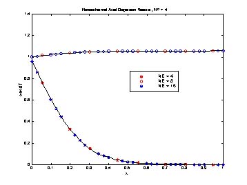
Figure 4. Axial Dispersion Non-isothermal Model, b = 0.056
The difficulty of the problem is enhanced when the heat of reaction (or activation energy) is higher.
This is achieved by increasing b or g. Solutions for
b = 0.2 are shown in Figure 5. Now the concentration profile is very steep and all the reactants are quickly consumed. The temperature rises to
its adiabatic value, 1 + b. Because of the steepness of the profile, 10 elements are used.
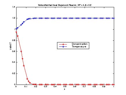
Figure 5. Axial Dispersion Non-isothermal Model, b = 0.2
Clearly this method can solve difficult problems.
Also, see the other solution methods: orthogonal collocation, finite difference, and initial value methods. (link)
Take Home Message: The method of orthogonal collocation on finite elements is ideally suited to problems involving axial dispersion, especially when the gradients are severe.