Orthogonal Collocation on Finite Elements
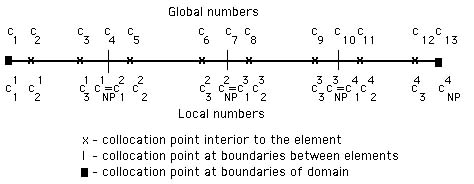
The orthogonal collocation method on finite elements is a useful method for problems whose solution has steep gradients, and the method can be applied to time-dependent problems, too. The method is a bit more complicated than others, since there are combined ordinary differential equations and algebraic equations. While the examples shown here use a uniform finite element mesh, non-uniform meshes are possible, and encouraged, when there are steep profiles in a known region of the domain (link). The arrangement of collocation points is shown in Figure 1.
Figure 1. Collocation Points for OCFE
We let
NE = the number of elements;
NP = the total number of collocation points per element;
NP2 = the collocations points interior to one element;
NT = NE (NP 1) + 1 = the total number of collocation points.
In Figure 1, NE is 4, NP is 4, and NT is 13.
Consider the case of diffusion in a slab for a case in which the diffusion coefficient depends upon the concentration. This might apply to diffusion through a polymer, for example.
![]()
The differential equation is expanded to give
![]()
The boundary conditions are typically
![]()
The equations are made nondimensional using the variables
![]()
The result is
![]()
It is convenient now to drop the primes.
![]()
The orthogonal collocation on finite elements divides the domain, 0 x 1, into finite elements, and sets the residual to zero at the collocation points interior to the elements (the points marked x in Figure 1). The elements are denoted by the superscript e (going from 1 to NE) and the points within an element are denoted by capital I or J (going from 1 to NP). Within the e-th element, we make the transformation
![]()
Then the differential equation becomes
![]()
in each element, and the boundary conditions become
![]()
The orthogonal collocation method is applied at each collocation point interior to the eth-element.
![]()
There are a total of NE*(NP1)+1 unknowns, where NE is the number of elements and NP is the degree of the polynomial within each element. The above equation gives NE*(NP2) equations to solve, leaving the need for NE+1 more equations. We obtain NE1 of these from the condition making the fluxes agree at element edges. Continuity of the function and first derivative between elements requires the condition
![]()
The function is continuous by virtue of assigning it only one value, regardless of whether it is the last point on one element or the first point on the next element. The diffusivities are the same at this point, since the concentration is the same. The continuity of first derivative is enforced using
![]()
This provides NE1 conditions. The last two conditions are the boundary conditions.
![]()
Now we have NE*(NP1)+1 equations. These equations are assembled into an overall matrix problem
![]()
The form of these equations is special, since most of the entries are zero. The shape of the matrix is shown in Figure 2. The center section of each block represents the residuals evaluated at the internal collocation points to an element. The first row and last row of the matrix represents the boundary conditions. The long rows adjoining the blocks represent the continuity conditions for the first derivative at the element edges.
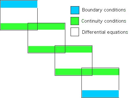
Figure 2. Matrix for Orthogonal Collocation on Finite Elements
The setup of the matrix is illustrated by taking the case of two elements of equal size x and D = constant, as shown in Figure 3.
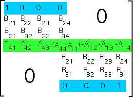
Figure 3. Matrix for OCFE with two equi-sized elements
The matrices A and B are the usual orthogonal collocation matrices (link). While the Newton-Raphson method could be used to linearize the equations, it is often easier to just evaluate the diffusivity at the prior iteration, i.e. use D(c(k)) when you solve for c(k+1). Then the iterations proceed by solving
![]()
The equations at the collocation points interior to an element are then
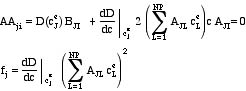
After the problem is solved, one item of interest is the flux at the side (which should be the same at each side). In OCFE, this is given by
![]()
![]()
In special situations it is possible to use one small element in one region, one large element in the rest of the region, where the solution is known, and solve problems analytically for asymptotic cases.
The case D(c) = 1 + 0.235 e2c is used for illustration. The diffusivity then varies by a factor of 1.8 over the domain. Typical solutions are shown in Figure 4 and the code is available. Using 2 elements and NP = 4 for a total number of 7 points is sufficient for a good solution, as confirmed by calculations with 4 elements (13 total points) and 8 elements (25 total points). It is possible to test convergence by increasing the number of elements (h-method) or the degree of polynomial in each element (p-method). Convergence of the flux with number of elements is shown in Table I.
Table I. Flux Values at x = 0 and x = 1, 4 collocation points per element
| NE | flux(0) | flux(1) | average | percentage error |
| 2 | –1.4310847 | –1.4310267 | –1.4310557 | 0.015 |
| 4 | –1.43125096 | –1.43124760 | –1.43124928 | 0.00073 |
| 8 | –1.43126053 | –1.43126045 | –1.43126049 | - |
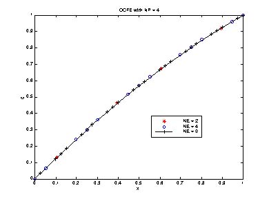
Figure 4. Nonlinear Diffusion with 2, 4, and 8 elements, 4 collocation points per element
Take Home Message: The method of orthogonal collocation on finite elements is ideally suited to problems involving steep gradients. This is demonstrated more clearly in other examples.