Derivation of Finite Difference Method for Problem II
Next we apply the finite difference method to Problem II. We evaluate the differential equations at the inner points, xi, i = 2,..., N1, and the boundary conditions at the points x1 and xN.
This completes the formulation of the finite difference method, at least for Problem II. We have replaced a differential equation, valid at all points, with a set of algebraic equations, valid at the grid points, with some error. Since each of the expressions for the derivatives has some error depending on ∆x, and the algebraic equations are written for specific ∆x, this means that the solution of the algebraic equations has an error (compared with the solution to the differential equation) that is also dependent on ∆x. Thus we have two important tasks: (1) solve the algebraic equations, and (2) determine or estimate the error in the solution to the differential equation.
The problem is solved for the case with
![]()
The complete problem statement is
![]()
A partial check on the results is obtained by using the program to solve the problem in the case with b = 0. In that case the solution is just a straight line, y = x (you should verify that this occurs with your program). All methods give the same results since they are all solving the same set of algebraic equations. The finite difference form of the equations is
![]()
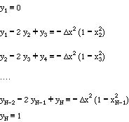
and the specific equations are
The results are summarized here for various ∆x in order to see the convergence as ∆x > 0. There are several methods available to solve the equations.
Analytic (link)
Mathematica, symbolic (link)
Matlab, using an LU decomposition or Gaussian elimination (link)
Excel, using successive substitution (link)
Excel, using 'Solver' (link)
The values of y(0.5) are plotted versus ∆x2 in the Figure BVP4 and are listed below.
Table BVP1. Values of y(0.5) for Finite Difference Method, Problem II
| ∆x | y(0.5) |
| 0.5 | 0.59375 |
| 0.25 | 0.58984375 |
| 0.125 | 0.588867188 |
| 0.0625 | 0.588623047 |
| 0.03125 | 0.588562012 |
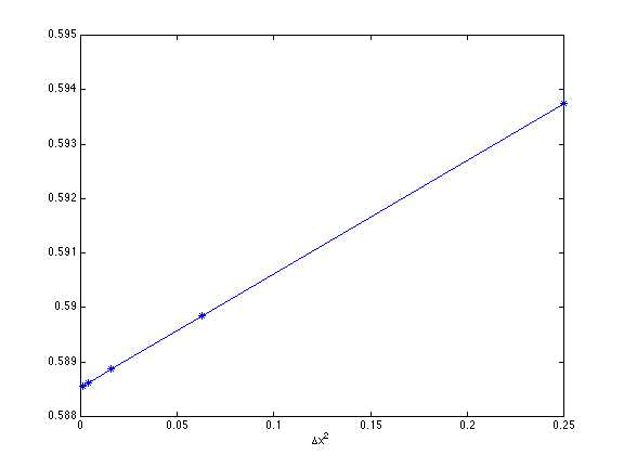
Figure BVP4. Solution to Problem II using Finite Difference Method; plotted versus ∆x2
Clearly for small ∆x the plot becomes linear; if the last two points are used extrapolate to zero the result is y(0.5) = 0.5885416667 (link). The fact that the curve is linear versus ∆x2 for small ∆x is one indication that we have done the calculation correctly. It shows that we have successfully implemented a second-order finite difference method to some problem. Whether we have done this for the right problem must be tested in the method (see the examples provided with each method). Here we can also compare the answer with the exact solution, since we know what it is. The solution to the Problem II can be found analytically (link)
![]()
Thus the exact answer is y(0.5) = 0.5885416667. The extrapolated finite difference solution gives the same answer, which verifies that we have solved the correct problem. The solution with ∆x = 0.03125 has an actual error of 0.000020, but the extrapolated solution is exact to 10 digits.
In summary, we have four types of evidence that show we have solved the right problem: (1) we obtained the exact solution to a simpler problem using the same computer code, (2) the answer to the real problem follows the expected truncation error, (3) in the method we verified that the appropriate functions were correct (see the examples), and (4) we compared with the exact solution. This last verification is not possible in more complicated cases, so it is important to learn the first three methods, and practice them on easy problems.