Problem II, Finite Difference Method, with MATLAB
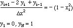
The problem to be solved is
![]()
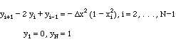
The finite difference formulation of this problem is
Rearrange the differential equation to the following form.
This set of equations can be written out in full.
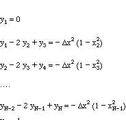
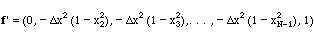
The equations are usually written in the following shorthand form.
![]()
where the vector f is
and the matrix AA is
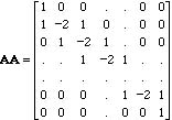
MOVIE Setting up Matrix Equations
These equations are applied here using MATLAB. The command file is shown below.
%solution to Problem II
dx = 1;
%This program will solve the problem five times, with decreasing delta-x
for kk=1:5
dx = dx/2;
n = 1 + 1/dx;
% Set up the matrix, aa, and right hand side function, f.
for i=2:n-1
x = dx*(i-1);
f(i) = dx*dx*(1+x*x);
for j=1:n
aa(i,j) = 0.;
end
aa(i,i-1) = 1;
aa(i,i) = -2;
aa(i,i+1) = 1;
end
% The matrix is special for the first and last row.
for j=1:n
aa(1,1) = 0;
end
f(1) = 0;
aa(n,n) = 1;
f(n) = 1;
% This is the Matlab command to solve AA y = f.
y = aa\f';
% Results are saved for later plotting.
nm = (n-1)/2 + 1;
y1(kk) = y(nm);
x1(kk) = dx*dx;
end
% The values of y(0.5) for different x are plotted versus x^2.
plot(x1,y1,'-*')
xlabel('x^2')
ylabel('y(0.5)')
How do we check our work? First, we remove the ';' from the statements, use ∆x = 0.25, and do the calculations by hand to compare with the MATLAB results. This insures that the calculations follow the equations given above. Next, we solve using successively smaller ∆x and see if the solution changes. The values of y(0.5) are plotted versus ∆x2 in the figure and are listed below.
| ∆x | y(0.5) |
| 0.5 | 0.59375 |
| 0.25 | 0.58984375 |
| 0.125 | 0.588867188 |
| 0.0625 | 0.588623047 |
| 0.03125 | 0.588562012 |
Clearly for small ∆x the plot becomes linear; if the last two points are used extrapolate to zero (Richardson extraplolation) , the result is y(0.5) = 0.5885416667. The fact that the curve is linear versus ∆x2 for small ∆x is one sign that we have done the calculation correctly. It shows that we have successfully implemented a second-order finite difference method to some problem; the problem is verified only by the line-by-line checking of the code.
MOVIE of extrapolation process.
Notice that this solution is also the same derived using Excel. That is as it should be, since we are solving the same equations.
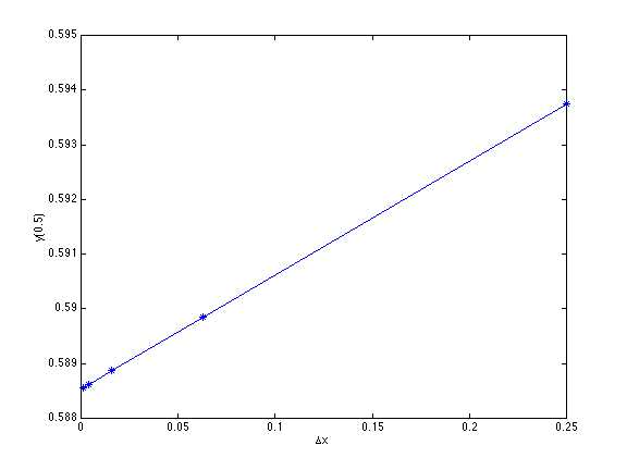
Figure. Convergence of solution with mesh size.
Take Home Message: Solve the same problem with different mesh sizes to determine the accuracy.