MWRheat

Application of the Method of Weighted Residuals to a heat transfer problem

We apply the Method of Weighted Residuals in five steps:

1. Expand the unknown solution in a set of basis functions, with unknown coefficients or parameters; this is called the trial solution.

2. Make the trial solution satisfy the boundary conditions (usually).

3. Define the residual.

4. Set the weighted residual to zero and solve the equations.

5. Examine the error by constructing successive approximations, and show convergence as the number of basis functions increases.

Let us apply MWR to a nonlinear heat transfer problem (link).

The first step is to expand the solution in a set of basis functions; here we choose powers of x as the basis set.

Next, we evaluate the solution at the boundaries.

To satisfy the boundary conditions requires

It is simpler to build that relation into the basis set by using c'0 = 0 and .

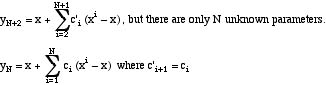
Thus, we define the N+2 approximation as

We redefine the coefficients (renumber them) to provide the N-th approximation in the new coefficients.

In step three we define the residual,

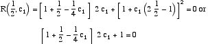
and in step four we apply the collocation method, and set the residual to zero at a set of points.

We choose as many points as we have unknowns. We solve this set of equations, and then repeat the process with more terms (step five).

For this case, and N = 1, the trial function is

and its derivatives are

The residual is then

The collocation point is taken as x = 0.5 (arbitrary, but logically in the mid-point of the interval).

Solving gives c₁ = 0.317.

For N = 2 the trial function is

and the collocation points are taken (again uniformly in the region) as

This time the weighted residuals (the residuals evaluated at the collocation points) give the following set of equations.

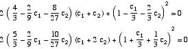
The solution is c₁ = 0.5992, c₂ = 0.1916. The two solutions are plotted in Figure 1 and are quite close to each other. The exact solution is plotted, too, for comparison. If we didn't have the exact solution (the usual case!), we would do higher approximations to see if our success holds.

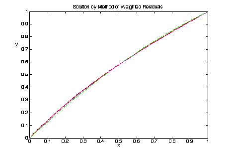
Figure 1. MWR Solution, N = 1 and 2 (green), and exact solution (red)

The solution can be examined, but only through the residual. Remember, we want the residual to be zero. The residual was defined as a function of x, with some constants, but now we know the constants. Thus, let us examine the residual as a function of x, using the known constants. This is done in Figure 2. The location of the collocation points is clear since the residual is zero there. (In this figure, for N = 2, we used the orthogonal collocation points, x₁ = 0.21132, x₂ = 0.78867 because it is easier to apply and more accurate.) We don't know whether having a residual as large as 1 elsewhere matters much or not. It is possible to derive error bounds (link) for the solution in terms of the residual, so we know we want the residual to be small, but don't know yet how small without experimentation. If we used N = 5, we get an even smaller residual (Figure 3). All three residuals are plotted on the same graph, Figure 4. With N = 5 the residual is much smaller than for N = 1 and N = 2; this lends credibility to the solution.

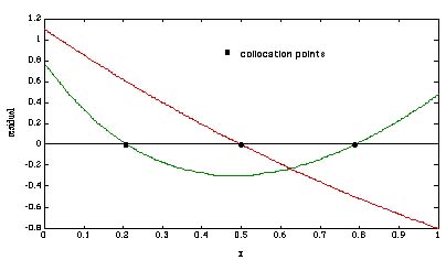
Figure 2. Residual for N = 1 and N = 2.

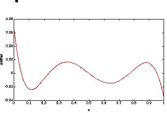
Figure 3. Residual for N = 5.

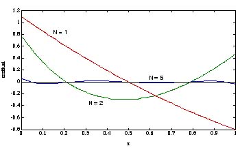
Figure 4. Residual for N = 1, 2 and 5.