IS/LM/FE: Increase in government spending

Reading: AB, chapter 10

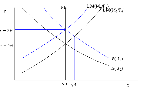
Consider the economy initially in general equilibrium with r* = 5% and full employment output Y*. Recall, in general equilibrium the labor market is in equilibrium, the goods market is in equilibrium (aggregate demand = aggregate supply) and the money market is in equilibrium. The initial price level is given by P₀. Now suppose the government increases its purchases of goods and services from G₀ to G₁. This increases the aggregate demand for goods and the IS curve shifts up and to the right. The level of demand is determined by the intersection between IS and LM and this is denoted Y^d. At the higher level of government spending the aggregate demand for goods is greater than the aggregate supply of goods, Y*. Firms will see their inventory of goods fall and they will respond by increasing prices. Also, workers will bargain for higher nominal wages to keep their real wage constant. As overall prices and wages rise, the LM curve will shift up and to the left and the real interest rate will rise. As r increases, interest sensitive spending (consumption and investment) falls as we move along the IS curve toward the new general equilibrium at r = 8%. At the new equilibrium, output is again Y* but the real interest rate and the price level are higher. Also, the higher amount of government spending has crowded out some private consumption and investment expenditure due to the higher real interest rate. The end result of the increased level of government spending is no increase in real output but the composition of demand has changed: more government spending and less private spending.