Derivation of the LM curve

Reading: AB, chapter 10, section 3.

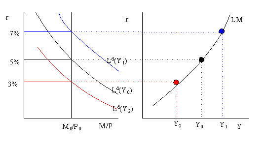
The LM curve, "L" denotes Liquidity and "M" denotes money, is a graph of combinations of real income, Y, and the real interest rate, r, such that the money market is in equilibrium (i.e. real money supply = real money demand). The graphical derivation of the LM curve is illustrated below.

The left-hand side of the graph illustrates money market equilibrium for a given level of Y. For example, when Y = Y₀ the equilibrium real interest rate is 5%. The right-hand-side of the graph gives the LM curve. The LM curve is plotted with the real interest rate on the vertical axis and real income (GDP) on the horizontal axis. Each point on the LM curve represents a money market equilibrium for a particular real interest rate and income pair (r, Y). For example, the money market equilibrium at (r=5%, Y=Y₀) is given by the black (middle) dot on the LM curve.

At a higher level of income, Y₁ > Y₀, the money demand curve shifts up and right and a new equilibrium occurs at r = 7%. This equilibrium is represented by the blue (upper) dot on the LM curve. Similarly, at a lower level of income Y₂ < Y₀ the money demand curve shifts down and left and a new equilibrium occurs at r = 3%. This equilibrium is given the by the red (lower) dot on the LM curve.

The above analysis shows that the LM curve is an upward sloping curve in the graph with r on the vertical axis and Y on the horizontal axis. Every point on the LM curve represents an intersection between the real money supply (M/P) and real money demand (L^d). The LM curve will shift whenever the variables we hold fixed, other than Y, in the money-supply/money-demand diagram change. These variable are M/P and ^e. In particular, if M/P increases holding expected inflation fixed then r falls in the money market and so the LM curve shifts down and right. Similarly, if expected inflation increases real money demand falls, lowering the interest rate, and the LM curve shifts down and to the right. Functionally, we represent the LM curve as

The (+) sign indicates that an increase in the variables shifts the LM curve down and to the right.