Reading: AB,
chapter 7, section 4; chapter 10 (all)
Last updated on February 19, 1996 .
Recall, inflation is simply the growth rate of some aggregate price index like the CPI or the GDP deflator. If P(t) denotes the aggregate price level in year t then, symbolically, annual inflation from year t-1 to year t is given as: = pi(t) = (P(t) - P(t-1))/P(t-1).
We build a link between money growth and inflation through our model of money market equilibrium. In money market equilibrium, real money supply is equal to real money demand: M/P = Ld(Y, i). If we assume that the aggregate price level is free to adjust to keep the money market in equilibrium then we can use the money market equilibrium condition to solve for the aggregate price level: P = M/Ld(Y, i). That is, the price level is directly related to the nominal money supply and to real money demand (which is a function of real income and the nominal interest rate).
Using the above relationship between the aggregate price level, nominal money supply and real money demand we may derive a link between inflation, growth in the money supply and growth in money demand. Inflation is just the growth rate of aggregate prices and from the relationship P = M/Ld(Y, i) we get, using the fact that the growth rate of a A/B is equal to the growth rate of A minus the growth rate of B, = %DP = %DM - %DLd(Y,i) (D = "delta"). That is, inflation is equal to the growth rate in the nominal money supply (controlled by the Fed) minus the growth rate in real money demand.
Notice that if the growth rate of the nominal money supply is equal to growth rate of money demand then inflation is equal to zero. Now money demand grows over time primarily because the real economy grows over time (average real growth is about 2.5% per year on average). As Y grows individuals consume more and thus need more money to conduct transactions. Since money demand is a function of both Y and i we can use a trick from calculus - the total derivative - to decompose the growth of money demand as follows: %DLd(Y,i) = eY*%DY + ei*%Di, where eY = income elasticity of money demand and ei = nominal interest rate elasticity of money demand. Economists estimate that eY is approximately 2/3, for the U.S., and that ei is approximately -1/10 so that money demand is much more sensitive to changes in income than to changes in the nominal interest rate. Further, the growth rate of the nominal interest rate is on average about zero (interest rate on average do not tend to go up or down). These data facts tell us that the nominal interest component does not contribute much to the growth rate of money demand and a reasonable good prediction model for inflation become:pi = %DP = %DM - (2/3)*%DY.
Suppose the Fed sets money growth, %M, equal to 6% per year, the annual real economic growth, %Y, is 3% and that the income elasticity of money demand is 2/3. Then our prediction for inflation is given by: = %M - (2/3)*%Y = 6% - (2/3)*3% = 4%.
The tables below show the relationship between actual inflation and money growth in low money growth countries and high money growth countries.
| Inflation in low money growth countries: 1986-1989 | ||
| Country | money growth (% per year) | inflation (% per year) |
| Chad | -2.1% | -2.7% |
| Switzerland | 4.1% | 1.8% |
| Belgium | 5.0% | 1.8% |
| France | 5.5% | 3.0% |
| United States | 7.0% | 3.6% |
| Inflation in high money growth countries: 1986-1989 | ||
| Country | money growth (% per year) | inflation (% per year) |
| Peru | 425% | 545% |
| Yugoslavia | 358% | 305% |
| Mexico | 71% | 82% |
| Poland | 47% | 68% |
| Nepal | 20% | 11.2% |
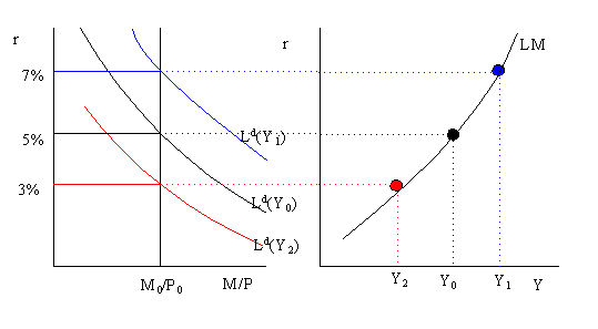
The LM curve, "L" denotes Liquidity and "M" denotes money, is a graph of combinations of real income, Y, and the real interest rate, r, such that the money market is in equilibrium (i.e. real money supply = real money demand). The graphical derivation of the LM curve is illustrated below.
The left-hand side of the graph illustrates money market equilibrium for a given level of Y. For example, when Y = Y0 the equilibrium real interest rate is 5%. The right-hand-side of the graph gives the LM curve. The LM curve is plotted with the real interest rate on the vertical axis and real income (GDP) on the horizontal axis. Each point on the LM curve represents a money market equilibrium for a particular real interest rate and income pair (r, Y). For example, the money market equilibrium at (r=5%, Y=Y0) is given by the black (middle) dot on the LM curve.
At a higher level of income, Y1 > Y0, the money demand curve shifts up and right and a new equilibrium occurs at r = 7%. This equilibrium is represented by the blue (upper) dot on the LM curve. Similarly, at a lower level of income Y2 < Y0 the money demand curve shifts down and left and a new equilibrium occurs at r = 3%. This equilibrium is given the by the red (lower) dot on the LM curve.
The above analysis shows that the LM curve is an upward sloping curve in the graph with r on the vertical axis and Y on the horizontal axis. Every point on the LM curve represents an intersection between the real money supply (M/P) and real money demand (Ld). The LM curve will shift whenever the variables we hold fixed, other than Y, in the money-supply/money-demand diagram change. These variable are M/P and e. In particular, if M/P increases holding expected inflation fixed then r falls in the money market and so the LM curve shifts down and right. Similarly, if expected inflation increases real money demand falls, lowering the interest rate, and the LM curve shifts down and to the right. Functionally, we represent the LM curve as

The (+) sign indicates that an increase in the variables shifts the LM curve down and to the right.
The IS curve represents all combinations of income (Y) and the real interest rate (r) such that the market for goods and services is in equilibrium. That is, every point on the IS curve is an income/real interest rate pair (Y,r) such that the demand for goods is equal to the supply of goods (where it is implicitly assumed that whatever is demanded is supplied) or, equivalently, desired national saving is equal to desired investment. The graphical derivation of the IS curve is given below.
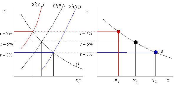
Consider an initial equilibrium in the goods market where r = 5% and income is equal to Y0. This equilibrium is illustrated in the graph on the right with r on the vertical axis and Y on the horizontal axis as the big black dot (middle dot). Now suppose Y increases to Y1 (say supply increases). This increase in Y shifts the desired savings curve down and right lowering the equilibrium real interest rate to 3%. The new equilibrium in the goods market with higher income and a lower real interest rate is illustrated in the graph on the right as the big blue dot (bottom dot). Similarly, if Y decreases from Y0 to Y2 then the savings curve shifts up and left and the equilibrium real interest rises. The new equilibrium in the goods market with lower income and a higher real interest rate is illustrated in the graph on the right as the big red dot (top dot). Notice that as income increases (decreases) the real interest must fall (rise) in order to maintain equilibrium in the goods market. This is the relationship that is represented in the downward sloping IS curve.
Every point on the IS curve represents an intersection between desired national saving and desired investment for some income/interest rate pair (Y,r). As such the IS curve is derived holding the determinants of saving and investment, other than Y and r, fixed. When these factors change the IS curve will shift. Since points on the IS curve represent points where aggregate demand is equal to aggregate supply any factor that increases the demand for goods and services will shift the IS curve up and to the right and any factor that decreases the demand for goods and services will shift the IS curve down and to the left. From the savings/investment diagram it follows that any shift of the savings or investment curve that increases the real interest rate, holding Y fixed, will shift up the IS curve. Functionally, the IS curve is represented as

Pluses (+) above the exogenous variables indicate that increases in the variables shift the IS curve up and to the right (increases demand).
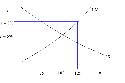
At r = 5% and Y = 100 the IS and LM curves intersect. At this point both the goods market and the money market are in equilibrium. This is called a general equilibrium since more than one market is in equilibrium simultaneously. If r = 8% and Y = 75 then the goods market is in equilibrium (on the IS curve) but the money market is not in equilibrium (off the LM curve). At r = 8%, Y is too low for the money market to be in equilibrium. To get to general equilibrium, r must fall and Y must rise (holding everything else fixed).
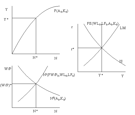
The above three diagrams represent general equilibrium in the labor market (labor demand = labor supply), goods market (desired saving = desired investment) and money market (money demand = money supply). Supply is determined by the interaction between the labor market and the production function. Equilibrium in the labor market determines the equilibrium real wage (W/P)* and the level of employment N*. Given the equilibrium level of employment the production function gives full employment output Y*. In the IS/LM diagram, we represent the full employment output (aggregate supply) restriction by the vertical FE (full employment) line. The FE line is vertical because full employment output does not depend on the real interest rate (it is assumed that the labor market and the production function are independent of the real interest rate). Points on the FE line represent equilibrium in the labor market. Exogenous factors that shift either the production function, labor demand or labor supply change the equilibrium level of Y* and thus shift the FE line. Functionally, we represent the FE line as
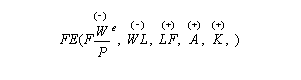
Pluses over the variables indicate that increases in the variables increase full employment outpout.
The intersection of IS, LM and FE at (r*, Y*) means that the labor market, goods market and money markets are in general equilibrium. At these values of r and Y there are not forces acting to move the economy from the equilibrium. Starting from an initial general equilibrium (intersection of IS, LM and FE), if either the IS, LM or FE line shifts the economy moves out of general equilibrium. The classical assumption is that when the economy is out of general equilibrium the aggregrate price level, P, adjusts so that the economy can move back to general equilibrium. Notice that when P changes the LM curves shifts. Thus the classical assumption is that the LM curve shifts in reaction to any shock that moves the economy away from general equilibrium.