Multiplier bootstrap and multi-stage estimator

Author: Yen-Chi Chen (University of Washington)
Date: 06/12/2026

This note is an introduction to the multiplier bootstrap for researchers and graduate students who know the empirical bootstrap but may not have much experience with the multiplier bootstrap.

We also discuss how to use a bootstrap method in a multi-steage procedure that the same data multiple times.

For readers who already know regression adjustment and doubly-robust estimator, you may jump to this section.

Short conclusion

We should use the coupled multiplier bootstrap, i.e., the weight $W_i$ of each observation stays the same throughout multiple stages. Do NOT use different weights at different stages for the same observation.

Introduction of multiplier bootstrap

The multiplier bootstrap is a popular method for assessing the uncertainty of an estimator from minimizing a (empirical) risk or solving a system of estimating equations.

We consider a simple regression model where our data consists of an univariate outcome $Y$ and a (possibly multivariate) covariate $X$ . Our goal is to estimate the conditional mean $m(x) = \mathbb{E}(Y|X=x)$ .
Our data consists of IID
$(X_1,Y_1),\cdots, (X_n,Y_n).$

Suppose we place a model on $m(x)$ that is indexed by a parameter $\theta$ , i.e., our model is $m_\theta(x)$ . Our goal is then to estimate $\theta$ from the data.
Consider the traditional least square estimator:
$\hat \theta_n = {\sf argmin}_\theta \, \frac{1}{n}\sum_{i=1}^n (Y_i - m_\theta(X_i))^2,$
where the quantity $\hat R_n(\theta) = \frac{1}{n}\sum_{i=1}^n (Y_i - m_\theta(X_i))^2$ is the empirical risk.
Under very mild conditions, we know that
$\sqrt{n}(\hat \theta_n - \theta^*) \overset{d}{\rightarrow} N(0, \Sigma),$
where $\theta^*$ is the parameter that minimizes the population risk
$\theta^* = {\sf argmin}_\theta R(\theta),\qquad R(\theta) = \mathbb{E}\left[(Y_1 - m_\theta(X_1))^2\right].$

Conventionally, we work out the score and Hessian of $R(\theta)$ and derive the asymptotic covariance matrix $\Sigma$ and construct an estimator of it. Note that this estimator often takes a form of $\hat \Sigma = \hat U \hat \Omega \hat U^T$ , so it is often known as a sandwich estimator.

The bootstrap procedure bypasses the need of doing the math to work out the estimator of $\Sigma$ . Instead, we use resampling technique to numerically compute an estimator of $\Sigma$ .

In particular, the multiplier bootstrap uses the following procedure to compute an estimator of $\Sigma$ :

Multiplier bootstrap

We generate IID weights $W_1,\cdots, W_n\sim {\sf Exp}(1)$ ^[1]
We compute the weighted least-square estimator:
$\hat \theta_n^* = {\sf argmin}_\theta \, \frac{1}{n}\sum_{i=1}^n W_i (Y_i - m_\theta(X_i))^2.$
Repeat the above two steps $B$ times, leading to
$\hat \theta_n^{*(1)},\cdots, \hat \theta_n^{*(B)}$
estimators.
We estimate the asymptotic covariance matrix using the sample covariance matrix of the $B$ bootstrap estimate:
$\hat \Sigma^*_B = \frac{1}{B} \sum_{b=1}^B (\hat \theta_n^{*(b)} - \bar \theta_{n,B})(\hat \theta_n^{*(b)} - \bar \theta_{n,B})^T, \qquad \bar \theta_{n,B} = \frac{1}{B}\sum_{b=1}^B \hat \theta_n^{*(b)}.$

The reason why multiplier bootsrtap work is that the added noises fluctuates the loss function, which mimicks the actual sampling randomness.
It is well-known that multiplier bootstrap works for a number of problems, not limited to regression. For instance, if we are fitting a parametric model to the data and we use the maximal likelihood estimator, we can use the multiplier bootstrap to estimate the asymptotic covariance matrix of our estimator.

A major benefit of the multiplier bootstrap (and other bootstrap variant) is that we do not need to work out the asymptotic covariance matrix and find an estimator to it. If we are able to compute the estimator once, we can easily modify the code with an extra for loop to assess the uncertainty.

Multiplier bootstrap versus empirical bootstrap

The empirical bootstrap samples with replacement of the original data to create a bootstrap sample and then compute the estimator using the bootstrap sample.

Both empirical and multiplier bootstrap are popular procedure in practice and in most cases, if one method works, we expect the other to work.
In terms of validity, empirical bootstrap is a lot easier to understand why it works:

Why empirical bootstrap works:

The bootstrap sample from the empirical bootstrap is IID from the empirical distribution of the original data. Since we know that the empirical distribution converges to the true CDF under very mild conditions, we expect the bootstrap sample behaves like a new sample from the target distribution.^[2]

When multiplier bootstrap is better than empirical bootstrap?

The multipler bootstrap, however, becomes a better approach when we have incomplete observations and the same size is small. We will dsicuss more about this later.

Multi-stage estimator

The story becomes more complicated when we have a multi-stage estimator. In particular, we will consider a very simple missing-at-random (MAR) scenario.

Suppose now the response variable $Y$ can be missing. So somtimes we only observe $X$ and sometimes we observe both $(X,Y)$ . To deal with missingness in our probability model, we introduce a binary response variable $R_i\in\{0,1\}$ such that $R_i=1$ if $Y_i$ is observed.

The (MAR) assumption assumes that the missingness of $Y$ is conditionally independent of the actual value of $Y$ given the covariate $X$ , i.e.,
$Y\perp R |X.$

Now we consider a very simple problem: estimating the marginal mean of $Y$ , i.e., we want to estimate $\mu \equiv \mathbb{E}(Y)$ .

Apparently, the naive estimator of using the mean value of observed $Y$ is not going to be consistent because this naive estimator
$\hat \mu_{\sf naive} = \frac{\sum_{i=1}^n R_i Y_i}{\sum_{j=1}^n R_j}\overset{P}{\rightarrow} \frac{\mathbb{E}(RY)}{\mathbb{E}(R)}\neq \mathbb{E}(Y)\equiv \mu.$

Under the (MAR), it is known that we can use a regression adjustment method for estimating $Y$ utilizing the fact that
$\begin{align*} \mu&\equiv \mathbb{E}(Y)\\ & = \mathbb{E}(RY + (1-R)Y)\\ & = \mathbb{E}[RY + (1-R)\mathbb{E}(Y|R,X)]\\ & = \mathbb{E}[RY + (1-R)\mathbb{E}(Y|X)]\\ & = \mathbb{E}[RY + (1-R)m(X)]. \end{align*}$
Therefore, the regression adjustment (RA) estimator suggests to use
$\hat \mu_{\sf RA} = \frac{1}{n}\sum_{i=1}^n R_i Y_i + (1-R_i) \hat m(X_i),$
where $\hat m(X_i)$ is an estimator of the outcome regression model $m(x) = \mathbb{E}(Y|X=x)$ .
Note that the regression model $m(x)$ is called a nuisance parameter.

Interpretation of RA estimator:

The regression adjustment estimator $\hat \mu_{\sf RA}$ has a simple interpretation: when $Y_i$ is observed, we use its observed value; when $Y_i$ is missing, we use the outcome regression model $\hat m(X_i)$ to predict its value.

If we use a parametric model like in the previous section, this estimator will be $\hat m(x) = m_{\hat \theta_n}(x)$ , where
$\hat \theta_n = {\sf argmin}_\theta \,\frac{1}{n}\sum_{i=1}^n R_i (Y_i - m_\theta(X_i))^2.$
Namely, we estimate the parameter using the complete data.

Caution

One should be careful that this RA estimator works only if our parameter of interest is the marginal mean $\mu \equiv\mathbb{E}(Y)$ . If the parameter of interest is other quantity, we have to use a different outcome regression model.

For $\hat \mu_{\sf RA}$ , how can we estimate its uncertainty?

The classical approach of doing asymptotic analysis still works and we are able to construct an estimator for asymptotic variance.
The bootstrap method also works here but we have to be careful since we are using data twice: the first time is to estimate the nuisance $m(x)$ and the second time

Continue: When multiplier bootstrap is better than empirical bootstrap?

When we have incomplete observations and sample size is small, multiplier bootstrap is generally better than the empirical bootstrap. This is because our bootstrap sample may not contain enoough observations to reliably estimate the nuisance (in the above example, the outcome regression model). When our copmlete observations have a small sample size, the empirical bootstrap sample may end up with no complete observations! So we cannot even produce a bootstrap estimate of the nuisance estimator. On the other hand, the multiplier bootstrap still works in this case.

Two versions of multiplier bootstrap

Recall that we have used data twice here:

The first time we use it for estimating the nuisance $\hat \theta_n$ for the regression model $m_{\hat \theta_n}(x)$ .
The second time we use it for the regression adjustment estimator $\hat \mu_{\sf RA}$ .
When using a parametric model for the nuisance, using data twice is generally not too much of a problem since the model class is not too complex^[3].

Now we want to use the multiplier bootstrap. A common question people asked is:

Since we have two estimators, should we use the same or different weights for each observation for the two estimators $\hat\theta_n$ and $\hat \mu_{\sf RA}$ ?

Method 1 (correct): coupled multiplier bootstrap (same weight).

The simple answer to this problem is: we use the same weight for the same observation in both stages.
Namely, we only generate one set of IID random weights $W_1,\cdots, W_n$ . Whenever $(X_i, Y_i, R_i)$ is used (in any stage), we always use the same weight $W_i$ .

Why do we have to use the same weight? This is because the bootstrap attempts to recover the uncertainty of the total estimator. In the original estimator, the same individual is used in both stages. This creates a dependency between the nuisance estimator and the regression adjustment estimator. We want the bootstrap to recover such dependency.

Method 2 (wrong): different weights for different stages.

If we use different weights, say $W_{i,1}$ when $(X_i, Y_i, R_i)$ is used for estimating $\hat \theta_n$ , and $W_{i,2}$ when $(X_i, Y_i, R_i)$ is used for $\hat \theta_{\sf RA}$ , this introduces independence between the two stages, so it underestimate the uncertainty in $\hat \theta_{\sf RA}$ .

Here is a simple simulation illustrating this problem; the code for this experiment is at the end of this note:

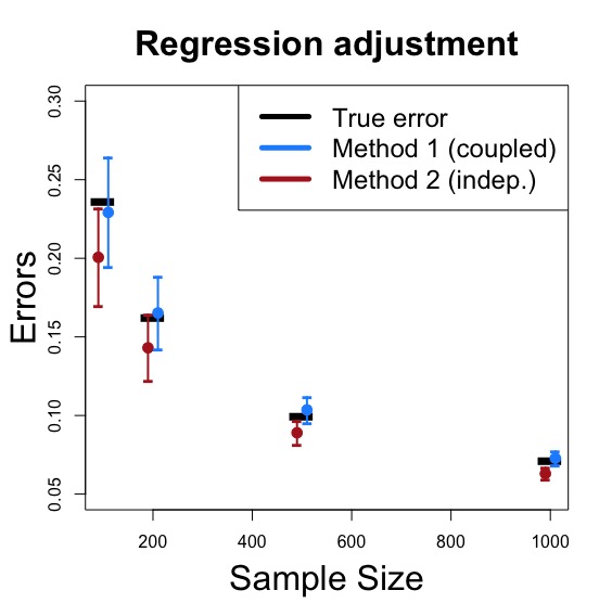
The blue lines indicating the result from the correct method: coupled multiplier bootstrap.
The brown lines indicating the result from the wrong method: independent multiplier bootstrap.

The black bar indicates the true errors. You can clearly see that the coupled multiplier bootstrap--we use the same weights for the two stages--recovers the true uncertainty while the independent multiplier bootstrap fails to recover it.

While here we consider the regression adjustment method, the same result occurs when we are using the inverse probability weighting estimator. The correct way of performing a multiplier bootstrap is to use the same weight in both stages.

Doubly-robust/one-step estimator

One may be wondering if the same biased result occurs for doubly-robust (DR) estimator. It turns out that if we are using DR estimators, using the different weights actually does not lead to a bias uncertainty estimate. However, using the correct procedure, the same weights across different stages, has a better finite sample performance.

Formally, the DR estimator is
$\hat \mu_{\sf DR} = \frac{1}{n}\sum_{i=1}^n \frac{Y_i R_i}{\pi_{\hat \beta}(X_i)} + m_{\hat \theta_n}(X_i) \left(1- \frac{R_i}{\pi_{\hat \beta_n}(X_i)}\right),$
where $m_\theta(x)$ is the regression model on $m(X) = \mathbb{E}(Y|X=x, R=1)$ and $\pi_\beta(x)$ is the propensity score model on $\pi(x) = P(R=1|X=x)$ . A common model for the propensity score is the logistic regresion: $\pi_\beta(x) = \frac{e^{\beta^Tx}}{ 1+e^{\beta^Tx}}$ and we estimate $\beta$ by a logistic regression of $R\sim X$ .

In this case, the estimator is a three-stage estimator since we use data three times:

First time: estimating the outcome model's parameter $\hat \theta_n$ .
Second time: estimating the propensity score model's parameter $\hat \beta_n$ .
Third time: computing the final estimator $\hat \mu_{\sf DR}$ .

We consider again two variants of the multiplier bootstrap:

[Method 1]: coupled multiplier bootstrap. Same weight $W_i$ for $i$ -th observation throughout the three stages.
[Method 2]: indpendent multiplier bootstrap. We have three independent weights $W_{i,1},W_{i,2}, W_{i,3}$ for each stage.

The following shows the result of using these two methods, assuming that both models are correct.

Result

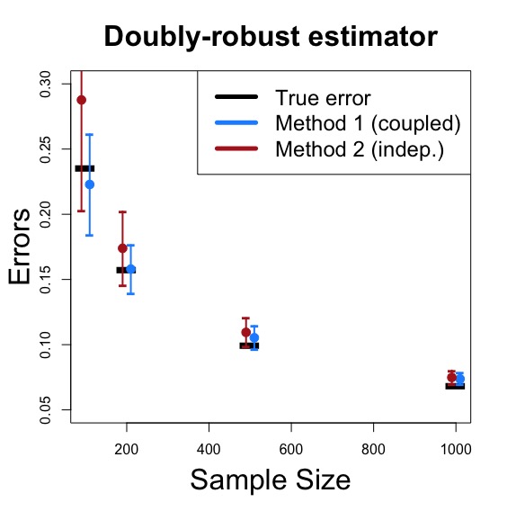
Now both methods are asymptotically valid when both models are correct while the coupled multiplier bootstrap is preferred since it approximates the actual uncertainty better.

Why?

The reason why both methods are valid is due to the fact that when both outcome regression and propensity score models are correct, the errors from these two nuisance models is negligible compared to the errors due to the final averaging process. Thus, while the independent multiplier bootstrap ignores the actual dependency of estimating the nuisance, such dependency contributes little to the overall uncertainty. So an inconsistent estimate of these uncertainties is fine.

However, despite the fact that both methods approximate the actual uncertainty, we still see that method 1, the coupled multipler bootstrap, is preferred since it better recovers the entire uncertainty, so it has a superior finite sample performance.

Appendix: R scripts

These R scripts are written by Gemini 3.1 pro.

For the regression adjustment estimator

# -------------------------------------------------------------------------
# 1. Data Generation
# -------------------------------------------------------------------------
set.seed(42)

n <- 1000
X <- runif(n, 0, 1)
E <- rnorm(n, 0, 1)

# True outcome
Y <- 3 + 4 * X + E

# Missingness mechanism (MAR)
# Note: Prompt stated P(M=1|Y) but formula only depends on X. 
# We implement the formula as given, which correctly satisfies MAR.
prob_missing <- exp(2 * X) / (1 + exp(2 * X))

# Let M = 1 denote missing, M = 0 denote observed
M <- rbinom(n, 1, prob_missing)

# Create the observed Y vector (NA where M == 1)
Y_obs <- Y
Y_obs[M == 1] <- NA

data <- data.frame(X, Y_obs, M)

# -------------------------------------------------------------------------
# 2. Point Estimation (Original Data)
# -------------------------------------------------------------------------

# [Outcome regression]
fit_or <- lm(Y_obs ~ X, data = data)

# [Propensity score] (Included per prompt, though not strictly needed for g-comp)
fit_ps <- glm(M ~ X, data = data, family = binomial(link = "logit"))

# [g-compute] Estimator
# Impute missing Y using the outcome regression
Y_imputed <- data$Y_obs
missing_idx <- which(data$M == 1)
Y_imputed[missing_idx] <- predict(fit_or, newdata = data[missing_idx, ])

# Point estimate for the mean of Y
mu_hat <- mean(Y_imputed)
cat("Point Estimate (mu_hat):", round(mu_hat, 4), "\n\n")

# -------------------------------------------------------------------------
# 3. Multiplier Bootstrap Setup
# -------------------------------------------------------------------------
B <- 500 # Number of bootstrap replicates

# Initialize vectors to store bootstrap estimates
boot_coupled <- numeric(B)
boot_indep <- numeric(B)

for (b in 1:B) {
  
  # Generate weights ~ Exp(1)
  W_coupled <- rexp(n, rate = 1)
  
  # For the independent variant, we need a second set of weights
  W_indep_OR <- rexp(n, rate = 1)
  W_indep_gcomp <- rexp(n, rate = 1)
  
  # =========================================================
  # Variant 1: Coupled Multiplier Bootstrap
  # =========================================================
  # 1. Weighted Outcome Regression
  # (lm automatically drops NAs, so we just pass the full data and weights)
  fit_or_coupled <- lm(Y_obs ~ X, data = data, weights = W_coupled)
  
  # 2. Impute missing values
  Y_imp_coupled <- data$Y_obs
  Y_imp_coupled[missing_idx] <- predict(fit_or_coupled, newdata = data[missing_idx, ])
  
  # 3. Weighted g-computation
  boot_coupled[b] <- sum(W_coupled * Y_imp_coupled) / sum(W_coupled)
  
  # =========================================================
  # Variant 2: Independent Multiplier Bootstrap
  # =========================================================
  # 1. Weighted Outcome Regression (using W1)
  fit_or_indep <- lm(Y_obs ~ X, data = data, weights = W_indep_OR)
  
  # 2. Impute missing values
  Y_imp_indep <- data$Y_obs
  Y_imp_indep[missing_idx] <- predict(fit_or_indep, newdata = data[missing_idx, ])
  
  # 3. Weighted g-computation (using W2)
  boot_indep[b] <- sum(W_indep_gcomp * Y_imp_indep) / sum(W_indep_gcomp)
  
}

# -------------------------------------------------------------------------
# 4. The "Gold Standard" Monte Carlo Truth
# -------------------------------------------------------------------------
# We simulate the true sampling variance by generating 1000 entirely new datasets

M_sims <- 1000
true_sampling_distribution <- numeric(M_sims)

for (m in 1:M_sims) {
  # Re-run the exact data generating process
  X_sim <- runif(n, 0, 1)
  E_sim <- rnorm(n, 0, 1)
  Y_sim <- 3 + 4 * X_sim + E_sim
  prob_missing_sim <- exp(2 * X_sim) / (1 + exp(2 * X_sim))
  M_sim <- rbinom(n, 1, prob_missing_sim)
  
  Y_obs_sim <- Y_sim
  Y_obs_sim[M_sim == 1] <- NA
  data_sim <- data.frame(X = X_sim, Y_obs = Y_obs_sim, M = M_sim)
  
  # Point Estimate
  fit_or_sim <- lm(Y_obs ~ X, data = data_sim)
  Y_imputed_sim <- data_sim$Y_obs
  missing_idx_sim <- which(data_sim$M == 1)
  Y_imputed_sim[missing_idx_sim] <- predict(fit_or_sim, newdata = data_sim[missing_idx_sim, ])
  
  true_sampling_distribution[m] <- mean(Y_imputed_sim)
}

true_se <- sd(true_sampling_distribution)

cat("\n--- The Moment of Truth ---\n")
cat("True Monte Carlo SE (Gold Standard):", round(true_se, 4), "\n")
cat("Coupled Multiplier Bootstrap SE:    ", round(se_coupled, 4), " (Accurate)\n")
cat("Independent Multiplier Bootstrap SE:", round(se_indep, 4), " (Underestimated)\n")

For the doubly-robust estimator

# -------------------------------------------------------------------------
# 1. Data Generation
# -------------------------------------------------------------------------
set.seed(42)

n <- 1000
X <- runif(n, 0, 1)
E <- rnorm(n, 0, 1)

Y <- 3 + 4 * X + E
prob_missing <- exp(2 * X) / (1 + exp(2 * X))

M <- rbinom(n, 1, prob_missing)
R <- 1 - M # R = 1 means Observed, R = 0 means Missing

Y_obs <- Y
Y_obs[R == 0] <- NA

data <- data.frame(X, Y_obs, M, R)

# -------------------------------------------------------------------------
# 2. Point Estimation (Doubly Robust)
# -------------------------------------------------------------------------

# [Outcome regression] m_hat(X)
fit_or <- lm(Y_obs ~ X, data = data)
m_hat <- predict(fit_or, newdata = data)

# [Propensity score] pi_hat(X) = P(R=1 | X)
fit_ps <- glm(R ~ X, data = data, family = binomial(link = "logit"))
pi_hat <- predict(fit_ps, type = "response", newdata = data)

# [Doubly Robust Estimator]
# Note: When R=0, Y_obs is NA. We use ifelse to safely evaluate 0 * NA as 0.
dr_terms <- m_hat + ifelse(data$R == 1, (1 / pi_hat) * (data$Y_obs - m_hat), 0)
mu_hat_dr <- mean(dr_terms)

cat("DR Point Estimate (mu_hat):", round(mu_hat_dr, 4), "\n\n")

# -------------------------------------------------------------------------
# 3. Multiplier Bootstrap Setup
# -------------------------------------------------------------------------
B <- 500

boot_coupled_dr <- numeric(B)
boot_indep_dr <- numeric(B)

for (b in 1:B) {
  
  # Generate weights ~ Exp(1)
  W_coupled <- rexp(n, rate = 1)
  
  # For independent, we draw separate weights for OR, PS, and Final Mean
  W_indep_OR <- rexp(n, rate = 1)
  W_indep_PS <- rexp(n, rate = 1)
  W_indep_FINAL <- rexp(n, rate = 1)
  
  # =========================================================
  # Variant 1: Coupled Multiplier Bootstrap (DR)
  # =========================================================
  # Fit models using the SAME weights
  fit_or_coupled <- lm(Y_obs ~ X, data = data, weights = W_coupled)
  # quasibinomial suppresses warnings for non-integer weights
  fit_ps_coupled <- glm(R ~ X, data = data, weights = W_coupled, family = quasibinomial) 
  
  m_hat_coupled <- predict(fit_or_coupled, newdata = data)
  pi_hat_coupled <- predict(fit_ps_coupled, type = "response", newdata = data)
  
  dr_terms_coupled <- m_hat_coupled + ifelse(data$R == 1, (1 / pi_hat_coupled) * (data$Y_obs - m_hat_coupled), 0)
  
  # Weighted mean
  boot_coupled_dr[b] <- sum(W_coupled * dr_terms_coupled) / sum(W_coupled)
  
  # =========================================================
  # Variant 2: Independent Multiplier Bootstrap (DR)
  # =========================================================
  # Fit models using INDEPENDENT weights
  fit_or_indep <- lm(Y_obs ~ X, data = data, weights = W_indep_OR)
  fit_ps_indep <- glm(R ~ X, data = data, weights = W_indep_PS, family = quasibinomial)
  
  m_hat_indep <- predict(fit_or_indep, newdata = data)
  pi_hat_indep <- predict(fit_ps_indep, type = "response", newdata = data)
  
  dr_terms_indep <- m_hat_indep + ifelse(data$R == 1, (1 / pi_hat_indep) * (data$Y_obs - m_hat_indep), 0)
  
  # Weighted mean using the third independent weight
  boot_indep_dr[b] <- sum(W_indep_FINAL * dr_terms_indep) / sum(W_indep_FINAL)
}

# -------------------------------------------------------------------------
# 4. The "Gold Standard" Monte Carlo Truth
# -------------------------------------------------------------------------
M_sims <- 1000
true_sampling_distribution_dr <- numeric(M_sims)

for (m in 1:M_sims) {
  X_sim <- runif(n, 0, 1)
  E_sim <- rnorm(n, 0, 1)
  Y_sim <- 3 + 4 * X_sim + E_sim
  prob_missing_sim <- exp(2 * X_sim) / (1 + exp(2 * X_sim))
  M_sim <- rbinom(n, 1, prob_missing_sim)
  R_sim <- 1 - M_sim
  
  Y_obs_sim <- Y_sim
  Y_obs_sim[R_sim == 0] <- NA
  data_sim <- data.frame(X = X_sim, Y_obs = Y_obs_sim, R = R_sim)
  
  # Fit on simulated data
  fit_or_sim <- lm(Y_obs ~ X, data = data_sim)
  fit_ps_sim <- glm(R ~ X, data = data_sim, family = binomial)
  
  m_hat_sim <- predict(fit_or_sim, newdata = data_sim)
  pi_hat_sim <- predict(fit_ps_sim, type = "response", newdata = data_sim)
  
  dr_terms_sim <- m_hat_sim + ifelse(data_sim$R == 1, (1 / pi_hat_sim) * (data_sim$Y_obs - m_hat_sim), 0)
  true_sampling_distribution_dr[m] <- mean(dr_terms_sim)
}

# -------------------------------------------------------------------------
# 5. Results
# -------------------------------------------------------------------------
se_coupled_dr <- sd(boot_coupled_dr)
se_indep_dr <- sd(boot_indep_dr)
true_se_dr <- sd(true_sampling_distribution_dr)

cat("--- DR Estimator Standard Errors ---\n")
cat("True Monte Carlo SE:                ", round(true_se_dr, 4), "\n")
cat("Coupled Multiplier Bootstrap SE:    ", round(se_coupled_dr, 4), "\n")
cat("Independent Multiplier Bootstrap SE:", round(se_indep_dr, 4), "\n")

The exponetial random variable can be replaced by other random variable with mean $1$ and variance $1$ . ↩︎
A caveat here is: we need the parameter of interest to be a smooth quantity in the sense that changing the underlying population distribution will smoothly changes the parameter of interest; this is formally known as the Hadamard differentiability. ↩︎
This is due to a property call Donsker class. If we use a nonparametric estimator for $\hat m$ , we generally need to avoid using data twice. ↩︎