CML

CML) is a set of procedures written in the GAUSS programming language (Schoenberg, 1995) for the estimation of the parameters of models via the maximum likelihood method with general constraints on the parameters

CML solves the general weighted maximum likelihood problem

where N is the number of observations, is a weight. is the probability of given , a vector of parameters, subject to the linear constraints,

the nonlinear constraints

and bounds

and are functions provided by the user and must be differentiable at least once with respect to .

CML finds values for the parameters in such that L is maximized using the Sequential Quadratic Programming method. In this method the parameters are updated in a series of iterations beginning with a vector of starting values. Let be the current parameter values. Then the succeeding values are

where is a direction vector, and a scalar step length.

Define

and the Jacobians

For the purposes of this exposition, and without loss of generality, we may assume that the linear constraints and bounds have been incorporated into G and H.

The direction, is the solution to the quadratic program

This solution requires that be non-negative definite (In practice, CML incorporates a slight modification in the quadratic programming solution which relaxes this requirement to positive semi-definite).

In practice, linear constraints are specified separately from the G and H because their Jacobians are known and easy to compute. And the bounds are more easily handled separately from the linear inequality constraints.

The SQP method requires the calculation of a Hessian, , and various gradients and Jacobians, , , and . CML computes these numerically if procedures to compute them are not supplied.

Descent Algorithms. The Hessian may be very expensive to compute at every iteration, and poor start values may produce an ill-conditioned Hessian. For these reasons alternative algorithms are provided in CML for updating the Hessian rather than computing it directly at each iteration. These algorithms, as well as step length methods, may be modified during the execution of CML.

Beginning with an initial estimate of the Hessian, or a conformable identity matrix, an update is calculated. The update at each iteration adds more ``information'' to the estimate of the Hessian, improving its ability to project the direction of the descent. Thus after several iterations the secant algorithm should do nearly as well as Newton iteration with much less computation.

There are two basic types of secant methods used in CML, the BFGS (Broyden, Fletcher, Goldfarb, and Shanno), and the DFP (Davidon, Fletcher, and Powell). They are both rank two updates, that is, they are analogous to adding two rows of new data to a previously computed moment matrix. The Cholesky factorization of the estimate of the Hessian is updated using the functions CHOLUP and CHOLDN.

BFGS is the method of Broyden, Fletcher, Goldfarb, and Shanno, and DFP is the method of Davidon, Fletcher, and Powell. These methods are complementary (Luenberger 1984, page 268). BFGS and DFP are like the Gauss-Newton method in that they use both first and second derivative information. However, in DFP and BFGS the Hessian is approximated, reducing considerably the computational requirements. Because they do not explicitly calculate the second derivatives, they are sometimes called ``quasi-Newton'' methods. While typically needing more iterations than the Gauss-Newton method, these approximations can be expected to converge in less overall time (though Gauss-Newton with analytical second derivatives can be quite competitive).

The secant methods are commonly implemented as updates of the inverse of the Hessian. This is not the best method numerically for the BFGS algorithm (Gill and Murray, 1972). This version of CML, following Gill and Murray (1972), updates the Cholesky factorization of the Hessian instead. The new direction is computed using a Cholesky solve, as applied to the updated Cholesky factorization of the Hessian and the gradient.

Line Search Methods. Define the merit function

where is the j-th row of G, is the -th row of H, is the vector of Lagrangean coefficients of the equality constraints, and the Lagrangean coefficients of the inequality constraints. The line search finds a value of that minimizes or decreases

where is a constant. Given and d, this is function of a single variable . Line search methods attempt to find a value for that decreases m. Several methods are available in CML, STEPBT, a polynomial fitting method, BRENT and BHHHSTEP, golden section methods, and HALF, a step-halving method.

Constraints. There are two general types of constraints, nonlinear equality constraints and nonlinear inequality constraints. However, for computational convenience they are divided into five types: linear equality, linear inequality, nonlinear equality, nonlinear inequality, and bounds.

Linear constraints are of the form

where A is an matrix of known constants, and B an vector of known constants, and the vector of parameters.

Linear constraints are of the form

where C is an matrix of known constants, and D an vector of known constants, and the vector of parameters.

Nonlinear equality constraints are of the form

where is the vector of parameters, and is an arbitrary, user-supplied function.

Nonlinear inequality constraints are of the form:

where is the vector of parameters, and is an arbitrary, user-supplied function.

Bounds are a type of linear inequality constraint. For computational convenience they are specified separately from the other inequality constraints.

Covariance Matrix of the Parameters. CML computes a covariance matrix of the parameters that is an approximate estimate when there are constrained parameters in the model (Gallant, 1987, Wolfgang and Hartwig, 1995). When the model includes inequality constraints, however, confidence limits computed from the usual t-statistics - dividing the parameter estimates by their standard errors - are incorrect because they do not account for boundaries placed on the distributions of the parameters by the inequality constraints. Confidence limits will have to be calculated therefore. Methods using inversion of the the Wald and likelihood ratio statistics are presented in the next section. The Wald method, however, requires an estimate of the covariance matrix of the parameters.

An argument based on a Taylor-series approximation to the likelihood function (e.g., Amemiya, 1985, page 111) shows that

where

Estimates of A and B are

Assuming the correct specification of the model plim(A) = plim(B), and thus

Without loss of generality we may consider two types of constraints, the nonlinear equality and the nonlinear inequality constraints (the linear constraints are included in nonlinear, and the bounds are regarded as a type of linear inequality). Furthermore, the inequality constraints may be treated as equality constraints with the introduction of ``slack'' parameters into the model:

is changed to

where is a conformable vector of slack parameters.

Further we distinguish active from inactive inequality constraints. Active inequality constraints have nonzero Lagrangeans, , and zero slack parameters, , while the reverse is true for inactive inequality constraints. Keeping this in mind, define the diagonal matrix, Z, containing the slack parameters, , for the inactive constraints, and another diagonal matrix, , containing the Lagrangean coefficients. Also, define representing the active constraints, and the inactive.

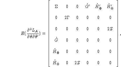
The likelihood function augmented by constraints is then

and the Hessian of the augmented likelihood is

where the dot represents the Jacobian with respect to , , and . The covariance matrix of the parameters, Lagrangeans, and slack parameters is the Moore-Penrose inverse of this matrix.

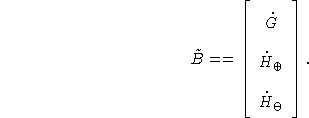
Usually we are interested only in the covariance matrix of the parameters, i.e., the upper left portion of the inverse associated with the parameters. This portion of the inverse can be produced using methods described in Hartmann and Hartwig (1995). For example, construct the partitioned array

Let be the orthonormal basis for the null space of , then the covariance matrix of the parameters is

Rows of this matrix associated with active inequality constraints may not be available, i.e., the rows and columns of associated with those parameters may be all zeros.

Heteroskedastic-consistent Covariance Matrix. CML computes a heteroskedastic-consistent covariance matrix of the parameters when requested. Define evaluated at the estimates. Then the covariance matrix of the parameters is .