Homework 4

Due Thursday, May 5, 2011, by 11:00pm PDT, by pushing to your bitbucket repository.

The goal of this homework is to gain some more practice with Fortran 90, modules, and Makefiles, and to start using OpenMP.

Before tackling this homework, you should read some of the class notes and links they point to. In particular, the following sections are relevant:

• OpenMP

Make sure you update your clone of the class repository before doing this assignment:

$ cd $CLASSHG
$ hg pull -u     # pulls and updates

You should also create a directory $MYHG/homeworks/homework4 to work in since this is where your modified versions of the files will eventually need to be.

Within in this directory you should have two subdirectories parta and partb for Part A and B below.

Numerical Quadrature

The Fortran files in $CLASSHG/codes/fortran/quadrature_hw4 implement the Trapezoidal rule for computing an approximation to the definite integral

\int_a^b f(x)\, dx

To do tests of the accuracy we will use functions for which we can compute the exact integral for comparison, but of course the point of numerical quadrature is to approximate integrals that cannot be computed exactly.

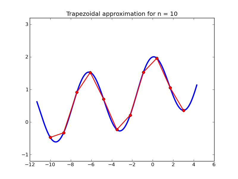
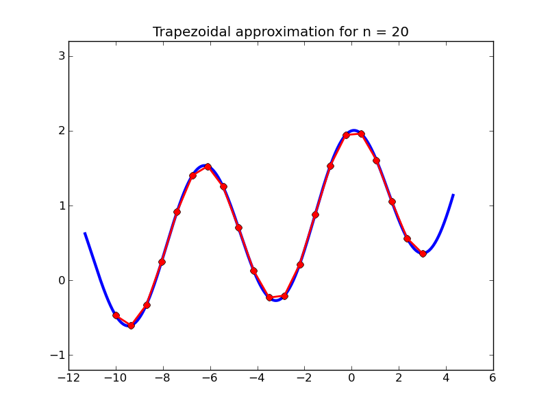
The Trapezoidal rule is a simple quadrature rule that is based on evaluating the function f(x) at n+1 points in the interval, approximating the function by a piecewise linear function connecting these function values, and computing the exact integral of this piecewise linear function. This is easy to do since on each of the n intervals between function values we only need to compute the area of a trapezoid. The figures below show examples where 10 and 20 intervals are used to approximate the interal

\int_{-10}^{3} \exp(x/10) + \cos(x)\,dx.

Let \Delta x = (b-a)/n and x_i=a + (i-1)\Delta x for i=1, 2, \ldots, n+1.

On interval number i from x_i to x_{i+1} the area is \frac {\Delta x} 2 (f(x_{i})+ f(x_{i+1})).

Summing this up from i=1 to n gives

\Delta x \left(\frac 1 2 (f(a) + f(b)) + \sum_{i=2}^n f(x_i) \right).

The trapezoidal rule is second order accurate, which means that if the function f(x) is sufficiently smooth then for small \Delta x (a large number of intervals), the error is proportional to (\Delta x)^2. So, for example, running the code in the directory $CLASSHG/codes/fortran/quadrature_hw4 gives:

$ make test
./testquad.exe
 How many intervals n?
20

Trapezoidal:    n =        20
   approx =  0.9434636084761E+01
   true =    0.9416892561216E+01
   error =   0.177E-01
   g was evaluated        21 times

$ make test
./testquad.exe
 How many intervals n?
200

Trapezoidal:    n =       200
   approx =  0.9417068999802E+01
   true =    0.9416892561216E+01
   error =   0.176E-03
   g was evaluated       201 times

Note that with n=200 the error is about 100 = 10^2 times smaller than with n=20.

Assignment:

Part A

1. There are much better methods than the Trapezoidal rule that are not much harder to implement but get much smaller errors with the same number of function evaluations. One such method is Simpson’s rule, which approximates the integral over a single interval from x_i to x_{i+1} by

   \int_{x_i}^{x_{i+1}} f(x)\, dx \approx \frac {\Delta x} 6 (f(x_i) + 4f(x_{i+1/2}) + f(x_{i+1})),

   where x_{i+1/2} = \frac 1 2 (x_i + x_{i+1}) = x_i + \Delta x/2.

   Add a subroutine simpson to the module quadrature_mod.f90 that implements Simpson’s rule. Note that when you sum the above expression over all i, you can combine some terms as was done in simplifying the Trapezoidal rule, so the result looks like

   \frac{\Delta x}{6}[f(x_1) + 4f(x_{3/2}) + 2f(x_2) + 4f(x_{5/2}) + 2f(x_3) + \cdots + 2f(x_n) + 4f(x_{n+1/2}) + f(x_{n+1})].

   Figure out a good way to evaluate this. Note that your program should evaluate the function only 2n+1 times for Simpson’s method. The code contains a counter that helps you check this.

   This method is 4th order accurate, which means that on fine enough grids the error is proportional to \Delta x^4. Hence increasing n by a factor of 10 should decrease the error by a factor of 10^4 = 10000. Check that your function works properly by experimenting with this on the function provided.

   Note: In finite precision arithmetic this asymptotic behavior is not seen if \Delta x is too small. Once \Delta x^4 is smaller than machine epsilon (around 2.d-16) you will not see any improvement by taking n larger.

   Have your main program print out results for Simpson’s rule in the same format as for Trapezoidal.

2. Modify your functions_mod.f90 so that the function being integrated is

   g(x) = \exp(x/10) + \cos(kx)

   where the wave number k is a module variable that is read in from the user by the main program (before the number of intervals) and then used in the definition of the function g(x).

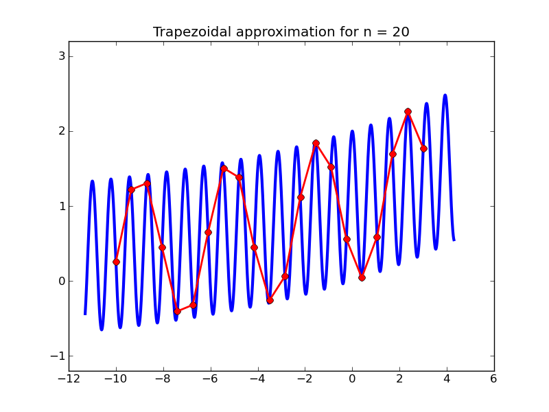
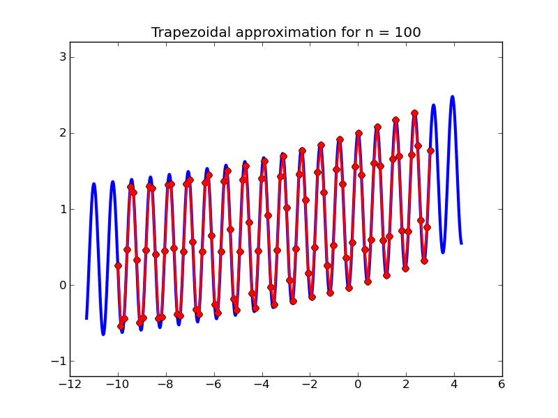
   So running your program should give results like:

   $ make test
   ./testquad.exe
    Wavenumber k?
   8.
    How many intervals n?
   20
   
   Trapezoidal:    n =        20
      approx =  0.1084939817273E+02
      true =    0.9582360287054E+01
      error =   0.127E+01
      g was evaluated        21 times
   
   Simpson:        n =        20
      approx =  0.9363491553954E+01
      true =    0.9582360287054E+01
      error =  -0.219E+00
      g was evaluated        41 times

   If k=1 this is the same function as before. For large k the function is highly oscillatory, making it difficult to integrate unless a sufficiently fine grid is used. For example, with k=8 as above the error is large when n=20, not surprising if you look at the plots below.

Part B

Now suppose we want to compute the integral with wave number k=10000. In order to get an accurate result we will have to take n very large. For this we might want an OpenMP version of the code.

1. Modify your code so that it uses OpenMP. Have nthreads be a variable of the module quadrature_mod.f90 that is set in the main program and used in the module in order to replace the do loops in trapezoid and simpson by omp parallel do loops. These loops must properly use reductions and private variables.

   Remove the call to evalfunc from the main program so you don’t have to worry about parallelizing this subroutine, which is just used to plot the function for plotting purposes.

   You might want to test your code on small values of k and n first.

2. Eventually test it with k=10000 and n = 50000000. Change the Makefile so that the time command is used when executing the code to determine how much time it takes. Hard wire these values of k and n into the main program rather than prompting the user, so the time to respond to the prompts doesn’t influence your results.

   So running the code should give something like:

   $ make test
   gfortran -c -fopenmp evalfunc_mod.f90
   gfortran -c -fopenmp functions_mod.f90
   gfortran -c -fopenmp quadrature_mod.f90
   gfortran -c -fopenmp testquad.f90
   gfortran -fopenmp evalfunc_mod.o functions_mod.o quadrature_mod.o testquad.o
   -o testquad.exe
   time ./testquad.exe
    Compiled with OpenMP
   Using   2 threads
   
   Trapezoidal:    n =  50000000
      approx =  0.9819716972423E+01
      true =    0.9819716972381E+01
      error =   0.415E-10
      g was evaluated  49444572 times
   
   Simpson:        n =  50000000
      approx =  0.9819716972380E+01
      true =    0.9819716972381E+01
      error =  -0.927E-12
      g was evaluated 147106801 times
   
          10.27 real        19.56 user         0.03 sys

   Note from the last line that 19.56 seconds of CPU time was used but the code ran in 10.27 seconds, which indicates that both cores were being used.

3. If you look at the number of times g was evaluated in the results above you will see that this is not what’s expected. There was a bug in my code that you might have missed too: The variable gcounter is not thread safe: both threads call g and update this counter independently and the result is somewhat random. Sometimes the value updated by one thread was in local cache and not seen by the other thread.

   Modify the code to keep a separate counter for each thread, or for more generality an array of length 8, by defining:

   integer :: gcounter_thread(0:7)

   which would allow nthreads up to 8. In the function g, use omp_get_thread_num to determine the thread number that made the call and update the corresponding element of the array. Output both values of the counter, so you will get output something like:

   $ make test
   time ./testquad.exe
    Compiled with OpenMP
   Using   2 threads
   
   Trapezoidal:    n =  50000000
      approx =  0.9819716972423E+01
      true =    0.9819716972381E+01
      error =   0.415E-10
      g was evaluated  25000002 times by thread 0
      g was evaluated  24999999 times by thread 1
   
   Simpson:        n =  50000000
      approx =  0.9819716972380E+01
      true =    0.9819716972381E+01
      error =  -0.927E-12
      g was evaluated  50000002 times by thread 0
      g was evaluated  49999999 times by thread 1
   
          10.27 real        19.56 user         0.03 sys

4. Your module testquad should also work if we provide a different main program and/or functions module for grading purposes.

5. Make sure your directory $MYHG/homeworks/homework4 contains the following subdirectories and files:

   • parta

     • testquad.f90
     • quadrature_mod.f90
     • functions_mod.f90
     • evalfunc_mod.f90 (unchanged from the original)
     • Makefile (unchanged from the original)
     • makeplot.py (unchanged from the original)

   • partb

     • testquad.f90
     • quadrature_mod.f90
     • functions_mod.f90
     • Makefile

When you are done, don’t forget to use the hg add, hg commit, and hg push commands to push these to your bitbucket repository for grading.