Traffic flow: the Lighthill-Whitham-Richards model
%matplotlib inline
%config InlineBackend.figure_format = 'svg'
import matplotlib as mpl
mpl.rcParams['font.size'] = 8
figsize =(8,4)
mpl.rcParams['figure.figsize'] = figsize
import matplotlib.pyplot as plt
import numpy as np
from ipywidgets import interact
from ipywidgets import widgets, FloatSlider
from utils import riemann_tools
from exact_solvers import traffic_LWR
In this chapter we investigate a conservation law that models the flow of traffic. This model is sometimes referred to as the Lighthill-Whitham-Richards (or LWR) traffic model (see (Lighthill, 1955) and (Richards, 1956)). This model and the corresponding Riemann problem are discussed in many places; the discussion here is most closely related to that in Chapter 11 of (LeVeque, 2002).
The LWR model
Recall the continuity equation:
$$\rho_t + (u\rho)_x = 0.$$Now we will think of $\rho$ as the density of cars on a road, traveling with velocity $u$. Note that we're not keeping track of the individual cars, but just of the average number of cars per unit length of road. Thus $\rho=0$ represents an empty stretch of road, and we can choose the units so that $\rho=1$ represents bumper-to-bumper traffic.
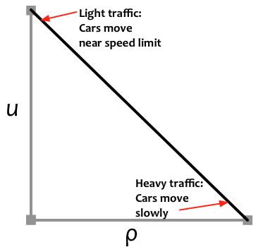
We'll also choose units so that the speed limit is $u_\text{max}=1$, and assume that drivers never go faster than this (yeah, right!) If we assume that drivers always travel at a single uniform velocity, we obtain once again the advection equation. But we all know that's not accurate in practice -- cars go faster in light traffic and slower when there is congestion. The simplest way to incorporate this effect is to make the velocity a linearly decreasing function of the density:
$$u(\rho) = 1 - \rho.$$Notice that $u$ goes to zero as $\rho$ approaches the maximum density of 1, while $u$ goes to the maximum value of 1 as traffic density goes to zero. Obviously, both $\rho$ and $u$ should always stay in the interval $[0,1]$.
Combining the two equations above, our conservation law says
$$\rho_t + (\rho (1-\rho))_x = 0.$$The function $\rho(1-\rho)$ is the flux, or the rate of flow of cars. Notice how the flux is zero when there are no cars and also when the road is completely full. The maximum flow of traffic actually occurs when the road is half full:
rho = np.linspace(0,1)
f = rho*(1.-rho)
plt.plot(rho,f,linewidth=2)
plt.xlabel(r'$\rho$'); plt.ylabel(r'flux $f(\rho) = \rho(1-\rho)$');
plt.ylim(0,0.3); plt.xlim(0,1); plt.grid(linestyle='--');
This equation is fundamentally different from the advection equation because the flux is nonlinear. This fact will have dramatic consequences for both the behavior of solutions and our numerical methods. But we can superficially make this equation look like the advection equation by using the chain rule to write
$$f(\rho)_x = f'(\rho) \rho_x = (1-2\rho)\rho_x.$$Then we have
$$\rho_t + (1-2\rho)\rho_x = 0.$$This is like the advection equation, but with a velocity $1-2\rho$ that depends on the density of cars. The value $f'(\rho)=1-2\rho$ is referred to as the characteristic speed. This characteristic speed is not the speed at which cars move (notice that it can even be negative, whereas cars only drive to the right in our model) Rather, it is the speed at which information is transmitted along the road.
Example: Traffic jam
What does our model predict when traffic approaches a totally congested ($\rho=1$) area? This might be due to construction, an accident or a red light somewhere to the right; upstream of the obstruction, cars will be bumper-to-bumper, so we set $\rho=1$ for $x>0$ (supposing that traffic has backed up to that point). For $x<0$ we'll assume a lower density $\rho_l<1$. This is another example of a Riemann problem: two constant states separated by a discontinuity. We have
$$ \rho(x,t=0) = \begin{cases} \rho_l & x<0 \\ 1 & x>0. \end{cases} $$What will happen as time goes forward? Intuitively, we expect traffic to continue backing up to the left, so the region with $\rho=1$ will extend further and further to the left. This corresponds to the discontinuity (or shock wave) moving to the left. How quickly will it move? The example below shows the solution (on the left) and individual vehicle trajectories in the $x-t$ plane (on the right).
def jam(rho_l=0.4,t=0.1):
    shock_speed = -rho_l
    shock_location = t*shock_speed
    fig, axes = plt.subplots(1,2,figsize=figsize)

    axes[0].plot([-1,shock_location],[rho_l,rho_l],'k',lw=2)
    axes[0].plot([shock_location,shock_location],[rho_l,1.],'k',lw=2)
    axes[0].plot([shock_location,1.],[1.,1.],'k',lw=2)
    axes[0].set_xlabel('$x$'); axes[0].set_ylabel(r'$\rho$');
    axes[0].set_xlim(-0.2,0.2); axes[0].set_ylim(0,1.1)
    traffic_LWR.plot_car_trajectories(rho_l,1.,axes[1]);
    axes[1].set_ylim(0,1); axes[0].set_title(r'$t= $'+str(t))
    plt.xlabel('$x$'); plt.ylabel(r'$t$');
    plt.show()

interact(jam,
         rho_l=FloatSlider(min=0.,max=0.9,value=0.2,description=r'$\rho_l$'),
         t=FloatSlider(min=0.,max=1.,value=0.2));
Speed of a shock wave: the Rankine-Hugoniot conditions
In the plot above, you see a shock wave (i.e., a discontinuity) that moves to the left as more and more cars pile up behind the traffic jam. How quickly does this discontinuity move to the left?
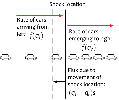
We can figure it out by putting an imaginary line at the location of the shock. Let $\rho_l$ be the density of cars just to the left of the line, and let $\rho_r$ be the density of cars just to the right. Imagine for a moment that the line is stationary. Then the rate of cars reaching the line from the left is $f(\rho_l)$ and the rate of cars departing from the line to the right is $f(\rho_r)$. If the line really were stationary, we would need to have $f(\rho_l)-f(\rho_r)=0$ to avoid cars accumulating at the line.

However, the shock is not stationary, so the line is moving. Let $s$ be the speed of the shock. Then as the line moves to the left, some cars that were to the left are now to the right of the line. The rate of cars removed from the left is $s \rho_l$ and the rate of cars added on the right is $s \rho_r$. So in order to avoid an accumulation of cars at the shock, these two effects need to be balanced:
$$f(\rho_l) - f(\rho_r) = s(\rho_l - \rho_r).$$This condition is known as the Rankine-Hugoniot condition, and it holds for any shock wave in the solution of any hyperbolic system!
Returning to our traffic jam scenario, we set $\rho_r=1$. Then we find that
$$s = \frac{f(\rho_l)-f(\rho_r)}{\rho_l-\rho_r} = \frac{f(\rho_l)}{\rho_l-1} = -\rho_l.$$This makes sense: the traffic jam propagates back along the road, and it does so more quickly if there is a greater density of approaching cars.
Example: green light
What about when a traffic light turns green? At $t=0$, when the light changes, there will be a discontinuity with traffic backed up behind the light but little or no traffic after the light. With the light at $x=0$, this takes the form of another Riemann problem:
$$ \rho(x,t=0) = \begin{cases} 1 & x<0 \\ \rho_r & x>0. \end{cases} $$In this case we don't expect the same discontinuity to propagate. Physically, the reason is clear: after the light turns green, the cars in front accelerate and spread out; then the cars behind them accelerate, and so forth. This kind of expansion wave is referred to as a rarefaction wave because the drivers experience a decrease in density (a rarefaction) as they pass through this wave. Initially, the solution is discontinuous, but after time zero it becomes continuous.
Similarity solutions
The exact form of the solution at a green light can be determined by assuming that the solution $\rho(x,t)$ depends only on $x/t$. A solution with this property is referred to as a similarity solution, because it is remains the same if we rescale both $x$ and $t$ by the same factor. The solution of any Riemann problem is, in fact, a similarity solution. Writing $\rho(x,t) = \tilde{\rho}(x/t)$ we have (with $\xi = x/t$):
\begin{align*} \rho_t & = -\frac{x}{t^2}\tilde{\rho}'(\xi) & \rho_x & = \frac{1}{t}\tilde{\rho}'(\xi) f'(\tilde{\rho}(\xi)). \end{align*}Thus \begin{align} \rho_t + f(\rho)_x = -\frac{x}{t^2}\tilde{\rho}'(\xi) + \frac{1}{t}\tilde{\rho}'(\xi) f'(\tilde{\rho}(\xi)) = 0. \end{align}
This can be solved to find \begin{align} f'(\tilde{\rho}(\xi)) & = \frac{x}{t} \end{align} or, since $f'(\tilde{\rho}) = 1-2\tilde{\rho}$, \begin{align} \tilde{\rho}(\xi) & = \frac{1}{2}\left(1 - \frac{x}{t}\right). \end{align} We know that the solution far enough to the left is just $\rho_l=1$, and far enough to the right it is $\rho_r$. The formula above gives the solution in the region between these constant states. For instance, if $\rho_r=0$ (i.e., the road beyond the light is empty at time zero), then
\begin{align} \rho(x,t) & = \begin{cases} 1 & x/t \le -1 \\ \frac{1}{2}\left(1 - \frac{x}{t}\right) & -1 < x/t < 1 \\ 0 & 1 \le x/t. \end{cases} \end{align}The plot below shows the solution density and vehicle trajectories for a green light at $x=0$.
def green_light(rho_r=0.,t=0.1):
    rho_l = 1.
    left_edge = -t
    right_edge = -t*(2*rho_r - 1)
    fig, axes = plt.subplots(1,2,figsize=figsize)
    axes[0].plot([-1,left_edge],[rho_l,rho_l],'k',lw=2)
    axes[0].plot([left_edge,right_edge],[rho_l,rho_r],'k',lw=2)
    axes[0].plot([right_edge,1.],[rho_r,rho_r],'k',lw=2)
    axes[0].set_xlabel('$x$'); axes[0].set_ylabel(r'$\rho$');
    axes[0].set_xlim(-1,1);  axes[0].set_ylim(-0.1,1.1)
    plt.xlabel('$x$'); plt.ylabel(r'$t$');

    traffic_LWR.plot_car_trajectories(1.,rho_r,axes[1],t=t,xmax=1.);
    axes[1].set_ylim(0,1)
    plt.show()

interact(green_light,
         rho_r=FloatSlider(min=0.,max=0.9,value=0.,description=r'$\rho_r$'),
         t=FloatSlider(min=0.,max=1.));
How can we determine whether an initial discontinuity will lead to a shock or a rarefaction?
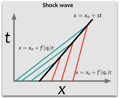
- Shocks appear in regions where characteristics overlap:
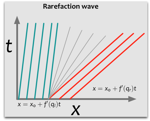
- Rarefactions appear in regions where characteristics are spreading out:
More precisely, if the value to the left of a shock is $\rho_l$ and the value to the right is $\rho_r$, then it must be that $f'(\rho_l)>f'(\rho_r)$. In fact the shock speed must lie between these characteristic speeds:
$$f'(\rho_l) > s > f'(\rho_r).$$We say that the characteristics impinge on the shock. This is known as the entropy condition, because in fluid dynamics such a shock obeys the 2nd law of thermodynamics.
On the other hand, if $f'(\rho_l)< f'(\rho_r)$, then a rarefaction wave results.
Interactive Riemann solution
The code in the next cell solves the Riemann problem for any inputs $(\rho_l,\rho_r)$. It returns a function reval(xi) that gives the value of the Riemann solution along any characteristic $\xi=x/t$.
def riemann_traffic_exact(rho_l,rho_r):
    r"""Exact solution to the Riemann problem for the LWR traffic model."""
    f = lambda rho: rho*(1-rho)
    if rho_r > rho_l: # Shock wave
        shock_speed = (f(rho_l)-f(rho_r))/(rho_l-rho_r)
        def reval(xi):
            if xi < shock_speed:
                return rho_l
            else:
                return rho_r
    else: # Rarefaction wave
        c_l  = 1-2*rho_l
        c_r = 1-2*rho_r

        def reval(xi):
            if xi < c_l:
                return rho_l
            elif xi > c_r:
                return rho_r
            else:
                return (1.-xi)/2.
    return reval
The cell below generates a plot that shows the Riemann solution, along with characteristics and vehicle trajectories, for any inputs $(\rho_l,\rho_r)$.
def c(rho, xi):
    "Characteristic speed."
    return 1.-2*rho

def plot_riemann_traffic(rho_l,rho_r,t):
    states, speeds, reval, wave_types = \
            traffic_LWR.riemann_traffic_exact(rho_l,rho_r)
    ax = riemann_tools.plot_riemann(states,speeds,reval,
                                    wave_types,t=t,
                                    t_pointer=0,extra_axes=True,
                                    variable_names=['Density']);
    riemann_tools.plot_characteristics(reval,c,axes=ax[0])
    traffic_LWR.plot_car_trajectories(rho_l,rho_r,ax[2],t=t,xmax=1.);
    ax[1].set_ylim(-0.05,1.05); ax[2].set_ylim(0,1)
    plt.show()

interact(plot_riemann_traffic,
         rho_l=FloatSlider(min=0.,max=1.,value=0.5,description=r'$\rho_l$'),
         rho_r=FloatSlider(min=0.,max=1.,description=r'$\rho_r$'),
         t=FloatSlider(min=0.,max=1.,value=0.1));
Other resources
Many other traffic flow models exist. Some of them are continuum models, like the one presented here, that model traffic density and velocity as an aggregate. Others are particle or agent models, that simulate individual vehicles. You can see simulations of the latter kind at http://www.traffic-simulation.de/routing.html. Shock waves and rarefaction waves naturally appear in such agent-based models too.