Advection
%matplotlib inline
import numpy as np
import matplotlib.pyplot as plt
import matplotlib as mpl
mpl.rcParams['font.size'] = 12
Conservation of mass
Imagine a fluid flowing in a narrow tube. We'll use $q$ to indicate the density of the fluid and $u$ to indicate its velocity. Both of these are functions of space and time: $q = q(x,t)$; $u=u(x,t)$. The total mass in the section of tube $[x_1,x_2]$ is
\begin{equation} \int_{x_1}^{x_2} q(x,t) dx. \end{equation}This total mass can change in time due to fluid flowing in or out of this section of the tube. We call the rate of flow the flux, and represent it with the function $f(q)$. Thus the net rate of flow of mass into (or out of) the interval $[x_1,x_2]$ at time $t$ is
$$f(q(x_1,t)) - f(q(x_2,t)).$$We just said that this rate of flow must equal the time rate of change of total mass; i.e.
$$\frac{d}{dt} \int_{x_1}^{x_2} q(x,t) dx = f(q(x_1,t)) - f(q(x_2,t)).$$Now since $\int_{x_1}^{x_2} \frac{\partial}{\partial x} f(q) dx = f(q(x_2,t)) - f(q(x_1,t))$, we can rewrite this as
$$\frac{d}{dt} \int_{x_1}^{x_2} q(x,t) dx = -\int_{x_1}^{x_2} \frac{\partial}{\partial x} f(q) dx.$$Under certain smoothness assumptions on $q$, we can move the time derivative inside the integral. We'll also put everything on the left side, to obtain
$$\int_{x_1}^{x_2} \left(\frac{\partial}{\partial t}q(x,t) + \frac{\partial}{\partial x} f(q)\right) dx = 0.$$Since this integral is zero for any choice of $x_1,x_2$, it must be that the integrand (the expression in parentheses) is actually zero everywhere! Therefore we can write the differential conservation law
$$q_t + f_x = 0.$$Here and throughout the book, we use subscripts to denote partial derivatives. This equation expresses the fact that the total mass is conserved -- since locally the mass can change only due to a net inflow or outflow.
Advection
In order to solve the conservation law above, we need an expression for the flux, $f$. The rate of flow is just mass times velocity: $f=u q$. Thus we obtain the continuity equation
$$q_t + (uq)_x = 0.$$In general, we need another equation to determine the velocity $u(x,t)$. In later chapters we'll exam models in which the velocity depends on the density (or other properties), but for now let's consider the simplest case, in which all of the fluid flows at a single, constant velocity $u(x,t)=a$. Then the continuity equation becomes the advection equation
\begin{align} \label{adv:advection} q_t + a q_x = 0. \end{align}This equation has a very simple solution. If we are given the density $q(x,0)=q_0(x)$ at time zero, then the solution is just
\begin{align} \label{adv:solution} q(x,t) = q_0(x-at). \end{align}Characteristics
Notice that the solution is constant along the line $x-at=C$, for each value of $C$. These are parallel, straight lines in the $x-t$ plane, with slope $1/a$.
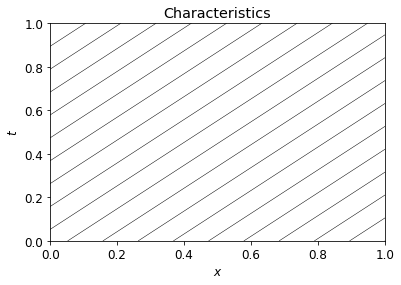
We can think of the initial values $q_0(x)$ being transmitted along these lines; we sometimes say that information is transmitted along characteristics.
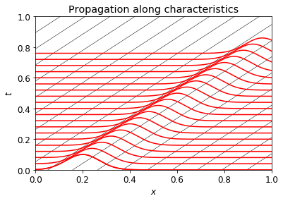
For more complicated hyperbolic problems, we may have multiple sets of characteristics, they may not be parallel, and the solution may not be constant along them. But it will still be the case that information is propagated along characteristics. The idea that information propagates at finite speed is an essential property of hyperbolic PDEs.
The Riemann problem
The Riemann problem consists of a hyperbolic PDE (like (\ref{adv:advection}) together with piecewise constant initial data consisting of two states. For convenience, we place the interface (or jump) at $x=0$ and refer to the left state (for $x<0$) as $q_l$ and the right state (for $x>0$) as $q_r$. We thus have
\begin{align} q_0(x) & = \begin{cases} q_l & x<0 \\ q_r & x>0. \end{cases} \end{align}For the advection equation, the solution to the Riemann problem is immediately obvious; it is simply a special case of (\ref{adv:solution}). The discontinuity initially at $x=0$ moves at speed $a$. We have
\begin{align} q(x,t) & = \begin{cases} q_l & x-at<0 \\ q_r & x-at>0. \end{cases} \end{align}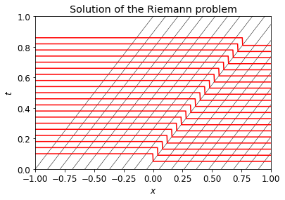
Notice how the initial discontinuity remains at the point defined by the characteristic coming from $x=0$ at $t=0$.
Code used to generate figures:
x = np.linspace(-1,1,20)
t = np.linspace(0,1,20)
a = 1.
for ix in x:
    plt.plot(ix+a*t,t,'-k',lw=0.5)
plt.xlim(0,1); plt.ylim(0,1); plt.title('Propagation along characteristics'); plt.xlabel('$x$');plt.ylabel('$t$');
xx = np.linspace(-1,1,1000)
q = 0.1*np.exp(-100*(xx-0.2)**2); plt.plot(xx,q,'-r');
spacing = 0.04
number = 20
for i in range(number):
    plt.plot(xx+spacing*i,q+spacing*i,'-r')

x = np.linspace(-1,1,20)
t = np.linspace(0,1,20)
a = 1.
for ix in x:
    plt.plot(ix+a*t,t,'-k',lw=0.5)
plt.xlim(-1,1); plt.ylim(0,1); plt.title('Solution of the Riemann problem'); plt.xlabel('$x$');plt.ylabel('$t$');
xx = np.linspace(-2,1,1000)
q = 0.05+0.05*(xx<0.)
spacing = 0.04
number = 20
for i in range(number):
    plt.plot(xx+spacing*i,q+spacing*i,'-r')
