Fuel-Gas Blending Benchmark
N. L. Rickera, C. J. Mullerb, I. K. Craigc
a Department
of Chemical Engineering, University of Washington, Seattle, WA, USA
b Sasol
Solvents RSA, Sasolburg, South Africa
c Department
of Electrical, Electronic, and Computer Engineering, University of Pretoria,
Pretoria, South Africa
Contents
· Downloadable MATLAB/Simulink code described in “Fuel-gas blending benchmark for economic performance evaluation of advanced control and state estimation”, submitted to the Journal of Process Control, 2011.
· Downloadable numerical results for the benchmark control strategy and an estimate of the optimal performance.
MATLAB/Simulink Considerations
The simulation was developed and tested in MATLAB release R2011b and Simulink version 8.0. It is unlikely to run in releases older than 2011a.
NOTE: To run the benchmark control strategy, your
MATLAB installation must include the Optimization Toolbox. The NLPcalc code uses the optimset and fmincon functions from this
Toolbox. If you are not licensed, the
simulation will terminate with an error
message.
To avoid this, replace the Controls block in the Simulink model with your
own control strategy.
Downloadable Archives
The downloadable materials are available in two ZIP archives, as follows
Benchmark_Model.zip The code and data required to run a simulation, consisting of the following five files
Blending_Challenge.mdl Simulink model file.
FG_Cleanup_Data.m MATLAB code that erases temporary files and Workspace variables at the end of a simulation.
FG_Initialize_Data.m MATLAB code that creates temporary files and Workspace variables needed to run a simulation.
Fuel_Gas_Blending_Data.mat MATLAB data file containing the information needed to run each of the three standard cases.
NLPcalc.m MATLAB code implementing the nonlinear program (NLP) solution employed by the benchmark control strategy. NOTE: your MATLAB installation must include the Optimization Toolbox or this code will generate an error message.
Benchmark_Results.zip The numerical results obtained using the benchmark control strategy and the estimated optimal control. This contains six files, two for each of the three standard cases
Results_Benchmark_i.mat where I = 1, 2, or 3
Results_Optimal_i.mat where I = 1, 2, or 3
See Benchmark Results for details of the file contents.
Simulating the Benchmark Strategy
The five model files must be placed in a directory on the MATLAB path. Open the Simulink model. The following screen shot shows the model’s block diagram on a Windows computer.
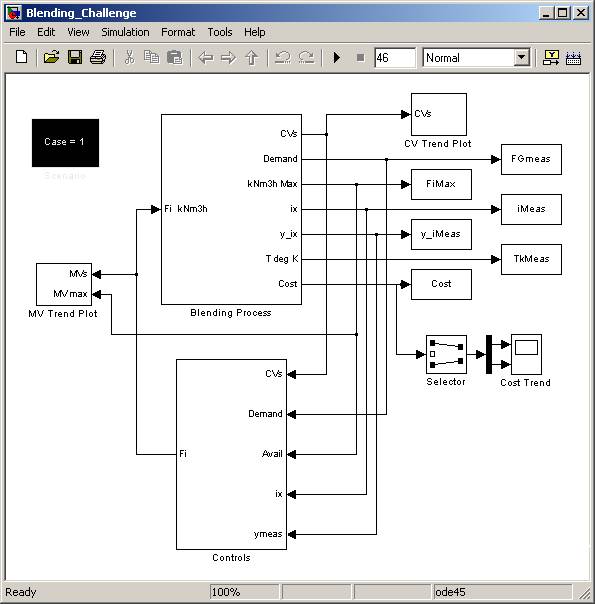
Model description
The block in the upper-left corner designates the case to be run. To change this, open it and edit the value (must be an integer from 1 to 3).
The Blending Process block simulates the process and its measurements. You may open it to examine the contents but should not make any changes.
The Controls block contains the benchmark control strategy. You can replace this with your own strategy.
The remaining blocks save numerical results and plot key variables as a function of time. You may modify or delete these blocks.
Running a simulation
To run the simulation, click the start button or use the Start command in the Simulation menu. A message box appears briefly to indicate the case being run. If this is incorrect, stop the simulation and enter the desired case.
NOTE: The simulation creates temporary data files in the MATLAB default directory and temporary variables in your Workspace. These should be deleted automatically when the model terminates.
A simulation of the 46-hour test scenario requires of order five minutes on a typical desktop computer. The main computational loads are integration of the plant’s state equations (by Simulink) and the Optimization Toolbox solution of the nonlinear program (NLP) employed by the benchmark strategy. The NLP is solved every 20 seconds of simulated time (the model’s base measurement interval).
By default, the simulation displays trend plots of the six feed flow rates (MVs), the four controlled variables (CVs), and the cost.
Simulation Signals
The signals appearing in the block diagram are listed below with brief descriptions. All update at the base sampling period, 20 seconds.
Cost Vector
containing the instantaneous cost, the penalty contribution to the
instantaneous cost, and the time-averaged cost.
For use as a performance metric, not for feedback to a
control strategy.
CVs Vector
containing the four controlled variables in the sequence: header pressure (kPa), HHV, WI, FSI.
FGmeas Scalar containing the measured
fuel-gas demand, kNm3/h.
FiMax Vector defining the availabilities or maximum
rates of the six feed gases, kNm3/h:
natural gas, reformed gas, hydrogen, nitrogen, tail gas 1, tail gas 2.
TkMeas Header temperature, K.
iMeas Spectrometer measurement
index. The spectrometer samples a gas
every two minutes. It requires 2 minutes
to complete its analysis, and then samples another gas in a pre-defined sequence. Thus, each of the five gases is measured
every 10 minutes.
The iMeas
value designates the gas for which a composition measurement is currently
available (in the y_iMeas signal). Possible iMeas
values are:
1 Natural gas
2 Reformed gas
5 Tail gas 1
6 Tail gas
2
7 Header
NOTE: The spectrometer can fail (with
probability 0.001). In that case, the iMeas value is negative.
y_iMeas Vector of measured gas mole
fractions corresponding to iMeas. If the measurement has failed (iMeas < 0), y_iMeas = 0.
MVs Vector containing the
desired flow rates for the six feed gases (same sequence and units as FiMax). In the block diagram,
the Controls block updates these
every 20 seconds.
Note: the simulation
samples iMeas and y_iMeas
every 20 seconds, as for all other signals, but the numerical values don’t
change until a new gas composition measurement becomes available (every 2
minutes).
Testing Your Strategy
The benchmark control strategy is contained within the Controls block. You must modify this or replace it with your strategy, which must define the Fi input to the Blending Process block (i.e., the MVs). Your strategy may use one or more of the output signals from the Blending Process block except for the Cost signal. Your strategy may not use the Blending Process internal data, or the data defining the disturbances and events.
The performance measure is the time-averaged cost at the end of the 46-hour test. This should be obtained for each of the three standard cases.
Benchmark Results
Numerical results obtained by the authors may be downloaded. Your machine’s numerical precision, software version, etc., may cause small deviations from these, but large differences indicate a problem in your installation. If you are unable to determine the cause, contact the authors with a description of the discrepancy including your machine type and the results of the MATLAB ver command.
For perspective, an estimate of the optimal strategy is also provided. This was calculated as described in Ricker et al. (2011).
To examine the result for a given case, load the corresponding file into your Workspace (by dragging the file into the Command window or using the MATLAB load command). NOTE: this creates variables having the names listed in Simulation Signals. WARNING: These will replace existing variables having the same names, if any.
Results: Format
By default, the model saves results in your Workspace. The downloadable results use the same variable names and formats.
With two exceptions, the variables are MATLAB double-precision arrays in which the 8281 rows represent time (46 hours at 20-second intervals), and each column is a variable. For example, FiMax contains six columns, one for each of the six feeds.
The exceptions are CV_Trend and MV_Trend, which are MATLAB structures created by a Simulink Plot block. For example, CV_Trend.time is the elapsed time (vector length 8281), CV_Trend.signals(1).values is a 8281x3 array in which the first column is the pressure, the second is its lower bound, and the third is its upper bound. CV_Trend.signals(2).values is a similar 8281x3 array for HHV, etc. The bounds are included because these appear in the default trend plot displays. MV_Trend.signals(1) to MV_Trend.signals(6) contain the six feed rates and their upper bounds. To see how CV_Trend and MV_Trend are created, open the CV Trend Plot and MV Trend Plot blocks in the block diagram.