DATA ACCESS
We have created several model extractions for people who are interested in analyzing the model output themselves. These are NetCDF files, so they have a lot of metadata like units and dimensions built-in, but you need to be able to work with them. Typically this would be using the python module xarray.
The current batch of extractions are for the model run called cas7_t0_x4b, which is our longest hindcast, going from 2012.10.07 through 2025.06.20. This has been replaced with another version of the model for the daily forecasts.
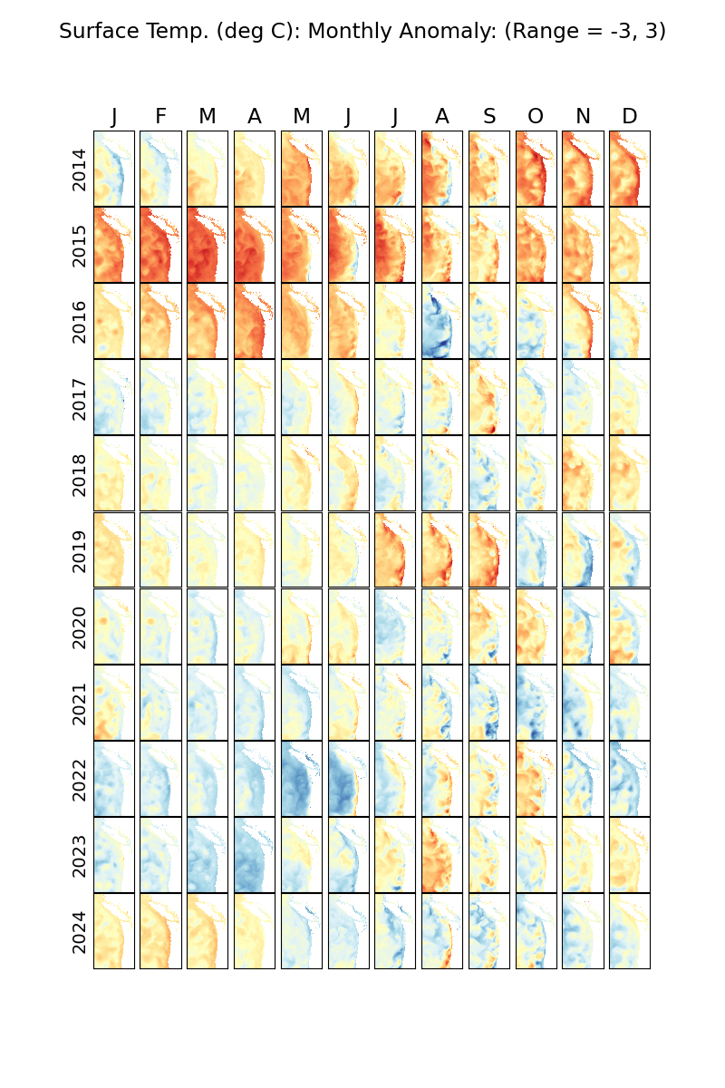
Some things to be aware of in cas7_t0_x4b: inside the Salish Sea NO3 is generally biased high, and bottom oxygen is sometimes biased low, also TIC (Total Inorganic Carbon) is biased a bit high, so if you calculate pCO2 it will be biased distinctly high in deep waters of the Salish Sea. Nonetheless, the output presented here can give useful information about seasonal and interannual variation. For example, here is a plot made from these files showing monthly SST anomalies over 11 years. The "Blob" Marine Heat Wave of 2014-2016 is clearly visible, especially in the early months of 2015.
Monthly-averaged 3-D fields are available using a URL of the form:
https://s3.kopah.uw.edu/cas7-t0-x4b/averages/monthly_mean_[2014-2024]_[01-12].nc
Sustitute a number for the year or month range, e.g. 2014 for [2014-2024].
Monthly climatologies of 3-D fields are available using a URL of the form:
https://s3.kopah.uw.edu/cas7-t0-x4b/climatologies/monthly_clim_[01-12].nc
The monthly climatologies are created by, for example, averaging all 11 years of January monthly-averaged fields to generate the "climatological" January over this time period. The plot was created by subtracting this climatology from each month to generate the anomaly.
Each file is about 780 MB.