NSCAT wind runs

NSCAT wind runs.


An idealized run like McCreary, Lee and Enfield (1989) (MLE)

This run has zero winds except for a single wind burst similar to a Tehuantepecker, blowing directly offshore (southward) from the Mexican coast at 95.45°W. This burst is exactly like that in MLE, with a half-sinusoid shape in x and t, and quarter sinusoid in y. The zonal width is 2.8° longitude, the meridional length is 4° latitude, and the wind blows for 6 days. The peak amplitude is 34.3 m/s, corresponding to 20 dynes/cm2 as in MLE. The model was initialized with flat isotherms and started from rest; the wind burst began immediately.

    Model fields of sea level, surface currents and SST at days 3, 6, 20, 40 (Figs 1-4 are comparable to Figs 9 and 10 of MLE).
  1. 3 days (center of wind burst)
  2. 6 days (end of wind burst)
  3. 20 days
  4. 40 days

    The following vertical sections show the sea level, layer thickness, temperature and vertical velocity fields in slices under the wind burst. The slices cut through the eddies as they are forming.
    Note that sea level and mixed layer thickness are unrelated, similarly vertical velocity and mixed layer thickness. (Total model upper layer thickness (thick line) is (inversely) related to sea level since this is a reduced gravity model). The mixed layer returns to nearly flat almost immediately after the winds stop (day 6).
    These features of the solution occur because the model mixed layer thickness is determined by Kraus-Turner physics. In this case, where the forcing is solely wind (no buoyancy), mixed layer thickness changes (dh/dt) are due entirely to stirring. Vertical velocity, which is due to horizontal divergence within the mixed layer, does not affect the interface depth.

  5. Vertical slices under the wind burst.

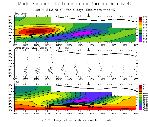
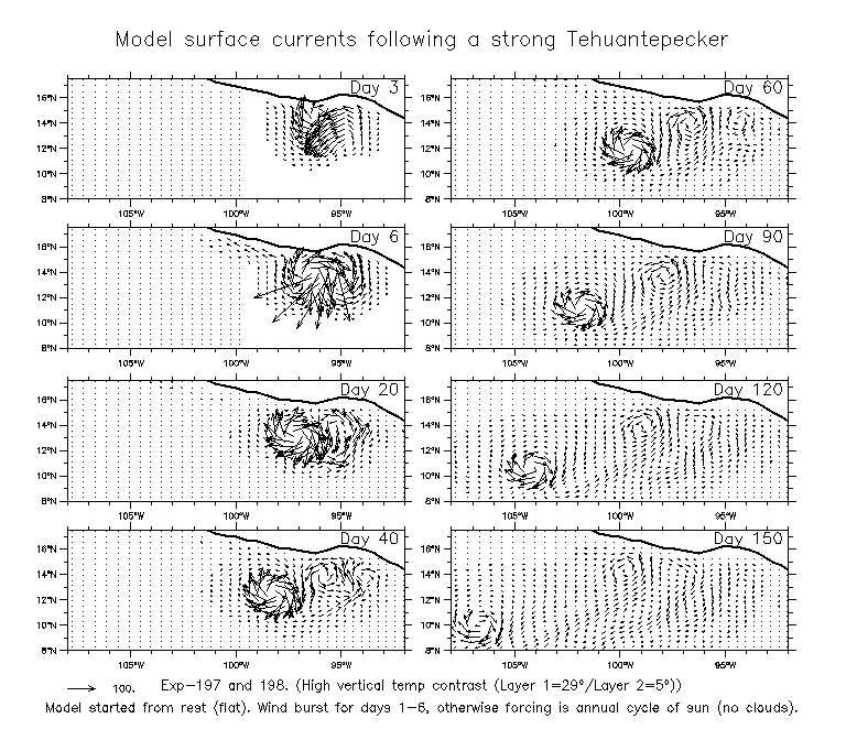
    Opposite to the observations and the MLE model, this model shows the anti-cyclonic eddy decaying and disappearing, while the cyclonic eddy remains and propagates west! The propagation speed is about 7 cm/s.

  6. The evolution of sea level over 150 days
  7. The evolution of surface current over 150 days

Here's the same figures from a run with a coarse grid (roughly 100 by 120km)

The forcing and initialization were identical to the fine-grid run above (in which the grid was roughly 20 by 20km). The vectors in figs 1-4 show the grid (vectors in fine-grid figs above were only every third vector in y). Note that the contour interval and vector lengthscale are much smaller in these coarse-grid figures.
Interestingly, although the eddies are quite weak and don't last very long, in this run the cyclonic eddy is the one that remains.
    Model fields of sea level, surface currents and SST at days 3, 6, 20, 40 (Figs 1-4 are comparable to Figs 9 and 10 of MLE).
  1. 3 days (center of wind burst)
  2. 6 days (end of wind burst)
  3. 20 days
  4. 40 days

  5. Vertical slices under the wind burst.

  6. The evolution of sea level over 150 days
  7. The evolution of surface current over 150 days

Here's the same figures from a run with a different vertical temperature structure

The forcing and initialization were identical to the main run above. The difference was that in the main run the vertical temperature structure was realistic, with T=29°C at the surface, decreasing slowly to 12°C at 400m. In particular, the constrast between the mixed layer and the layer below was only from 29°C to 28.5°C. In the run shown below, all the layers below the ML were set to 12°C.
    Model fields of sea level, surface currents and SST at days 3, 6, 20, 40 (Figs 1-4 are comparable to Figs 9 and 10 of MLE).
  1. 3 days (center of wind burst)
  2. 6 days (end of wind burst)
  3. 20 days
  4. 40 days

  5. Vertical slices under the wind burst.


Here's the same figures from a run with an even larger vertical temperature contrast (28°C to 5°C)

The forcing and initialization were identical to the main run above, but in this run the constrast between the mixed layer and the layer below was from 29°C to 12°C.
    Model fields of sea level, surface currents and SST at days 3, 6, 20, 40 (Figs 1-4 are comparable to Figs 9 and 10 of MLE).
  1. 3 days (center of wind burst)
  2. 6 days (end of wind burst)
  3. 20 days
  4. 40 days

  5. Vertical slices under the wind burst.

  6. The evolution of sea level over 150 days
  7. The evolution of surface current over 150 days

Comparing model runs with various forcing during Jan 96-Jun 97

  1. Model surface height in Jul 96, Oct 96, Jan 97, Apr 97
  2. As above for SST
  3. Model surface height along 13°N
Are these bands Tehuantepecker eddies?
Look again. Note (in the third figure) that the westward-propagating bands, particularly the 1997 one that corresponds to the apparent eddy in the first two figures, are emitted from the boundary. Also note that this occurs in the FSU run, which has no mountain-gap winds.

A few checks of interest to no one but me

    Check the EC winds used for spinup:
  1. Zonal wind time series compared to the original EC winds
  2. Meridional wind time series compared to the original EC winds

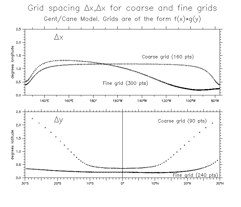
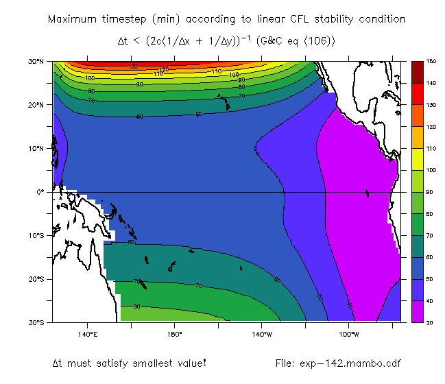
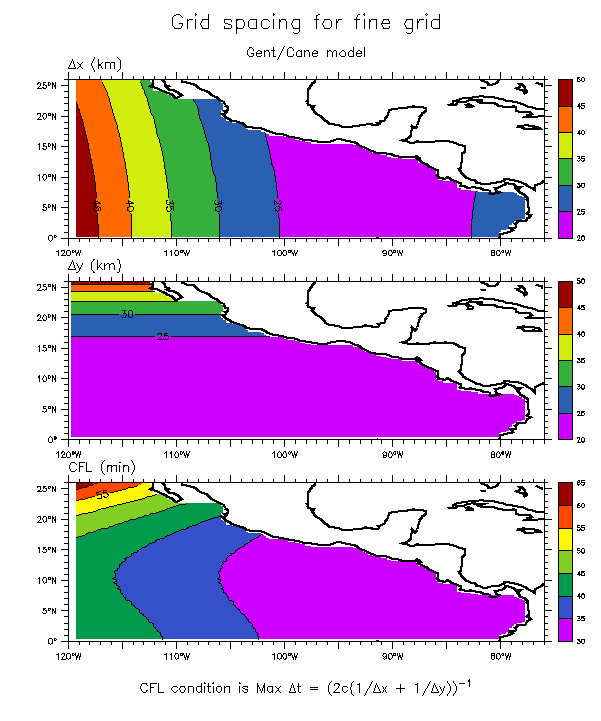
    Check the grid spacing:

  3. Grid spacing for the coarse and fine grids
  4. CFL condition for the fine grid
  5. Grid and CFL condition for fine grid (detail near Central America)