Tutorial One:

Price determination and the One-Price law.

Markets bring buyers and sellers together.    That’s the easy part.  The hard part consists in distinguishing where one market starts and another ends.  Buyers and sellers transact all kinds of goods in numerous places, some of which are defined by their physical locale, like a supermarket or flea market, and some of which, like NASDAQ or the used car market, are dispersed, brought together only by wires or mail or couriers.   Local markets work within he context a larger markets, as for example we can imagine the market for Boeing workers is embedded in the local Seattle market, and this in turn is embedded in the larger U.S. labor market.

Economists are inclined to model markets as jurisdictions in which a single price prevails.  They do this even though we rarely observe these uniform prices.  Thus, while we’ll borrow the economists’ basic model, we do have to recognize that it is just that, a model which abstracts from the actual details one sees every day.  Though the standard model simplifies the world, it does not do so arbitrarily.   Market behavior gives rise to predictable incentives, one of which is to take advantage of price differences wherever this is cost feasible.   The results is that when we observe different prices for the same good, we are inclined to look for, and can usually identify, market barriers.

Why should transaction prices tend to move together in a single market?  This question is at the heart of the one price law.  We expect that when prices are low in one market and high in another, buyers and sellers who can costlessly move from one market to another--a big assumption—take advantage of the situation by buying in the low priced market and selling in the high priced one.  An individual who performs both these functions at the same time is said to be “arbitrage” markets, pocketing the price difference between the buy price and the sell price.  If enough people catch on to this game, then increased selling activity causes prices to fall in the high priced market.  Likewise, pressures to increase price develop in the previously low priced market as an increasing number of buyers compete for the available goods.  In the absence of barriers to trade, economists expect prices for identical goods in the two markets become equal. Of course, there is almost always some barrier to doing business in a new place and consequently arbitrage or buying low and selling high seldom eliminates all price differences. We merely expect that active and free competition narrow prices differentials, thus justifying the simplified market model in which all transactions occur at the same price. 

That we seldom see uniform prices for long anywhere does not refute the economists’ “one price law” anymore than does the observation that water clearly exists at a variety of levels, refute the saying that water “seeks its own level” by flowing downward.  Comparison between water movements and markets is instructive.  Think of markets like water basins that overflow into secondary basins if inflows exceed drainages.  Yet whether the overflow results in a common level between creating one large basin or two separate levels (like the two prices in separate economic markets) depends both upon the physical contours of the land and the flows in and out of the basins.  In studying economics, we are often interested in discovering how the land is shaped because it helps us to understand prices, which, as we’ll see, constitute crucial flow valves that channel economic activity.  For some economists, there is no greater goal than getting the price right.  Their reasoning is that competitive prices reveal the value of resources, and only if the information contained in the price of goods is reliable will these resources be put to the best use.  Failing to do get prices right results in waste—putting high valued goods in low valued uses--which in economic analysis is practically a cardinal sin.  In discussing the Soviet Union, Marshall Goldman gives us an example in which meat prices were kept so low that that meat was fed to chickens as feed, a clearly inefficient use of resources when grains always require less resources to grow than livestock.

The existence of price differentials would mean that prices do not properly indicate the value of resources unless the costs of moving goods from low priced areas exceeds the value to be derived in the high priced ones.  It is therefore not simply a matter of idle speculation why prices vary in different markets.   That software programmers generally earn less in India than the U.S. suggest a problem.  Why don’t American producers higher more programmers in India, and in the process raise their wages to the level of U.S. programmers?  Likewise, if programmers are so expensive in the U.S., why don’t we encourage foreign programmers to immigrate here, reducing the cost of production?  From a simple observation, we have now suddenly entered the policy domain, in which we can imagine ways in which the economist’s claim for efficiency competes with other social values.   This is but one of an almost infinite number economic issues that arise when we start to examine the operation of markets and the existence of price differentials.   Economics throws light on these kinds of issues precisely because it makes important claims.  First, it claims to know how people will behave in response to the incentives embedded in price signals.  Second, many practitioners claim that those responses will produce greater wealth (less waste, more efficiency) so long as policy makers and market participants do not add arbitrary and unnecessary barriers that obstruct the arbitrage principle.

We’ll step back for a moment from these kinds of larger problems to consider the less noticed case in which the prices an individual faces varies in a given transaction.  The point of this exercise is simply to demonstrate how pervasive the problem of price differentials is, and why we sometimes expect them to persist with not great efficiency concerns.  When you buy a soda or coffee from a vender you are frequently given a choice that looks something like the following.

16 oz for $2.00

20 oz for   2.25

In this case the price per ounce of your drink varies as you purchase more.    If the consumer upgrades to the larger size that the price of the last four ounces is twenty-five cents, or on average ounce is priced at a little more than 11.25 cents.   If the 16 ounce size is purchased, the price of each ounce averages out to be 12.5 cents. Normally, these kinds of discrepancies produce opportunities to arbitrage.  In short, a person can buy the larger size drink at the lower per ounce price.   Necessarily, there exists some incentive to buy the larger size drink and sell what one doesn’t need to the next comer at a price between the 11.25 and 12.5.   However for most people that incentive will be offset by the costs of resale (waiting, finding customers, stocking, etc), which we may anticipate to be greater than the difference of one and a quarter cent.  Perhaps it is too extreme to say that no one will arbitrage this market, because some families or friends may well share two or thee drinks rather than buying individual smaller portions.  So at this margin we would see that among families the costs of arbitrage may be small, but we will not expect many individuals to become entrepreneurs buying low and selling high at this margin.

The point is that we see in this example how transactions may be linked.  To the extent that goods sell at different prices, incentives are created to arbitrage the related markets by re-trading cheap goods into more expensive markets.  When arbitrage is cost-effective, transactions are linked in a web of markets.  In the limit, re-trading is costless; prices in once separate markets converge to a single level.  In this sense, transactions are nested in larger set of market relations wherein people may take advantage of price differentials.  When we look at more important questions than those involving the price of an extra four ounces of soda, questions such as price, race or sex discrimination, unequal development, or price dumping, what we’ll be trying to understand is what natural and artificial barriers exist and how they raise the costs of market arbitrage that might otherwise connect disparate transactions.

Demand and Supply.

Having noted these concerns we may now simplify our world by envisioning markets as places in which buyers and sellers come together to establish a market price.  While we know that in more instances than not, no single price exists for all transactions in a given good, we also know that the existence of multiple prices encourage arbitrage that pushes prices toward a uniform level.

Demand.  Markets depend on the interactions of buyers and sellers whose desires are represented by the forces of demand and supply.   Individual buyers have different valuations of goods, and when these individuals are combined together in a market, the quantity demanded tends to slope down with respect to price.  That is, as price declines, consumers generally desire more.  In a market consisting of two consumers, if one individual values a good at $5 and the other values it at $4, then market demand looks like this:

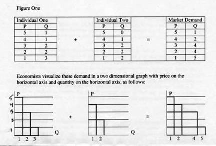
In the graphs above we are seeing how individuals respond to lower prices.  They do not all respond in the same way, and every lower price does not necessarily induce an increase in quantity purchased.  However, for the market at as whole, we are apt to see a clearer downward sloping pattern because it is made up of many individuals having similar responses.

It is worth noting that when consumers are induced to buy additional units of a good they may be bridging or partially arbitraging markets.  That is, generally consumers are not interested in a specific good but rather a type of experience.  For example, going to a restaurant, consumers are interested in eating and not necessarily in eating one particular thing.  Instead they often base part of their choices on the price of a menu item –we may only speculate how often hosts choke back their disappointment when their guests don’t do this.  What is happening is that diners are looking for a food experience and they may be inclined to substitute one type of food for another (that is to say that the market is really for food and, not just for pasta or some other specific good).

 If consumers substitute easily across foods, then demand for a particular item is very responsive.  Economists measure consumer responsiveness by calculating price or “own” elasticity, which is defined as the percentage change in the quantity that is demanded when price changes by one percentage.   The more elastic is demand for a good, the more the consumer considers prices in related markets important to his or her decisions.    To say that elasticity is measured to be 4 is to say that the quantity demanded of a good by consumers will change 4 % for every one per cent change in price.    When consumers find it possible to substitute one good for another they are arbitraging markets by seeking their satisfaction in a cheaper market.. [1]

Price elasticity indirectly measures the ease with which individuals substitute products in one market for products in another.  Taking cheese, for example, we can compare the demand curve, one for a person who imagines many good substitutes at comparable prices and another for a person who finds few acceptable alternatives.  We note that the consumer who loves many foods is expected to have a flatter demand curve while the cheese lover’s demand is steeper.  The former we say is relatively elastic—demand will vary widely with price because the purchaser can easily be convinced to buy other goods--while the later is regarded as relatively inelastic. One thing to note here is that while demand always slopes downward--at lower prices some consumers buy more—consumers are more responsive to price changes for some goods than for others. All that is happening is the consumers are arbitraging markets by buying where they can attain consumption satisfaction cheapest.  This point is illustrated in the graph below showing relative elasticities.

 

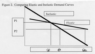
In Figure 2 we see two demand curves that intersect each other.  If we let P1 be the price at which they intersect we can see that for the same movement to price P2 quantity responds more on the flatter (and therefore relatively elastic) graph.

Elasticity can be important to market analysts for a number of reasons, two examples of which will hopefully be sufficient.  If government officials are trying to raise revenues, they may want to add taxes onto the price of specific goods.  However, if they fail to account for the degree to which consumers have elastic responses to price increases, they may drastically overstate tax revenues.  For example, Washington DC is surrounded by two independent states, and when local authorities there placed additional taxes on gasoline, they were caught short.  Local residents substituted Maryland and Virginia gas for DC gas and total tax revenues declined.  Separately, we may consider how a retailer views an increase in price.  She expects that she will lose some sales by raising price, but only if demand is elastic and sales fall by more than price increases will she lose revenue, making the price increase self-defeating.  In such ways sellers, buyers and policy makers find it important to know how easily markets easily are bridged.

We gain a fuller understanding of market relationships if we consider variables other than those of the good in question to change.  We may consider a market for milk.  If the consumer believes that alternative markets are available, and are cost effective, then the demand for milk is elastic.  By alternatives, we can imagine a host of potential markets from water, juice, pop, to various sellers located at some distance in time or space.  So given that consumers have a sense of what the prices in the markets they believe are relevant, then we can draw a graph of their demand for milk at a particular location for a particular point in time, as in the graph below.

Figure 3:  Typical Demand

The Demand Curve is drawn under the assumption that all other relevant variables are held constant.

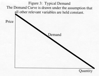
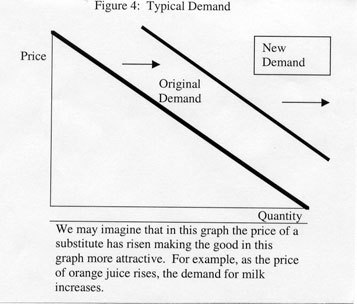
To draw that graph, prices in all the related markets must be known and held constant.  Clearly, if consumers believe that milk will go sale at next week at Jenny’s Market, then at least some of them will be inclined to wait for the price reduction there and shift purchases forward.     Consequently, if our graph of demand has only two axes, one describing prices and the other quantity of a particular good over some fixed period of time, then it can only be drawn under the assumption that everything else that affects demand is held constant.   If something does change, like the expectation that prices fall in the future, then we must draw a new relationship and the old one disappears.  So we can imagine that demand for a good shifts or changes when the price of substitutes change.  One such substitute is an identical good at another location, another is a good possessing some of the characteristics that made original good valuable, and a third involves the same good sold at a future time.

Before going further it is helpful to restate some main findings and to suggest some new ones.

1)   Consumer demand responds to price.  Higher prices reduce quantity demanded and lower prices increase it.

2)   Consumer demand also depends on the availability of goods whose consumption provides a substitutable form of satisfaction.

3)   Consumer demand is more elastic when substitutes are available at competitive prices.

4)   Demand curves are drawn under the assumption that prices of related goods are held constant.

5)   When the prices of related goods change we may conceptualize this by redrawing the demand curve (changing or shifting the demand relationship).

6)   The responsiveness of consumer demand to other variable besides its own price can also be measured as a type of elasticity.

The elasticity measure can be helpful in graphing supply and demand.  Normal price elasticity (known as “own” elasticity) is measured as the percentage change in quantity demanded of a good for each percentage change in the price of the good under consideration.  “Cross” elasticity, however, is measured as the percentage change in quantity that is demanded for each percentage change in the price of another good.  We now have a way of defining when markets are bridged.  In particular, when a change in the price of one good has a measurable positive effect on another, then these goods are substitutes.  In other words, if prices for juice rise by 5% and the quantity of milk demanded increases by 2% consumers view these goods as substitutes. When cross elasticity is positive, it means that a price change in one market leads to a shift of demand in another market and that this shift will have the same direction.  For example if the price of orange juice goes down, the demand curve for milk decreases.

By analogy we can define the elasticity of demand for other factors such a complements or income.  When the “cross” elasticity between one good and the price of another good is negative, consumers view these goods as complements.  Complementary goods are consumed together in order to achieve consumer satisfaction.  Oil and new cars—particularly big gas-guzzlers-- may be complements.  If the price of oil goes up, not only does the demand for oil go down, but so too would the demand for big cars.  So cross elasticity here means that when price of one good goes up, the demand curve for a related good decreases.  While we may suspect that goods are either substitutes or complements, we can verify this by obtaining measurements of cross elasticity of demand to see if they are positive (substitutes) or negative (complements).

Income elasticity is yet one more measure of how demand responds to changes in consumer income.  Normally we expect that when income rises, demand will increase.  This would mean income elasticity is positive.  For a few goods, income elasticity will be negative which means that these goods are considered inferior or that as individuals become wealthier they substitute away from these goods.  Other variables do affect demand but they are harder to quantify and thus elasticity coefficients for things like price expectation in the future, fashion or taste, are not easy to measure.  Conceptually, however, they work the same way.

The Table below suggest how demand changes when quantifiable variables change and what elasticity means in these situations.

Variables	Relationship	Elasticity Measure	Elasticity Measure
Price of a good	P up Q demanded down P down Q demanded up	Own	> 1 elastic; < 1 inelastic
Price of Related Goods (substitute)	Subs P up Demand up	Cross	Positive
Price of Related Good(complement)	Complement P up; Demand down	Cross	Negative
Income (normal goods)	Income up Demand up	Income	Positive
Income (inferior goods)	Income up Demand down	Income	Negative
Price expectations	Expect higher P, Demand Down	None	Positive

Supply.   The principles of supply are easy to digest.  Sellers are motivated by profit and higher prices make selling profitable for more individuals.  Thus as prices go up, two things are likely to happen. First, more sellers are willing to sell a given object.  Some existing sellers will be willing to sell more units of a good because they stock themselves with more units that may be more expensive to procure.  In the oil market for example, we know that Saudi Oil is some of the cheapest oil to produce and North Sea oil some of the most expensive.  Thus if prices went very low, Norway and Britain might not find it advantageous to sell oil, but when prices are higher all producers have an incentive to dig deeper and use more intensive oil recovery techniques to bring more costly oil to market.  While we could go through an exercise similar to the demand example showing how two individuals’ behavior can be added together, that can be left for an exercise.  Here it is only necessary to show that market supply from several sellers produces an upward sloping supply curve like that shown in figure 5 below.

 

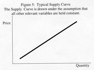
Supply, like demand, is drawn under the assumption that anything other than the price of the good for sale that influences seller behavior is held constant.  Sellers, like buyers, encounter several arbitrage possibilities.  Sellers, like farmers, have choices about what to produce with their existing plant and capacity.  So wheat farmers may find that if the price of corn rises, they’d prefer to produce and sell for the more expensive market.   Consequently, the behavior of supplier is affected by the prices available by pursuing different alternatives (the best alternative forgone is called a sellers opportunity cost).   When the price of alternatives goods that sellers may produce rise, they may choose to sell less.  It is the price of inputs, however, that generally drives supply.  When these rise, then supply falls (shifts left).    Likewise, if new technology develops, production is generally less costly and supply increases (shifts right).  Besides the intangible factors of production, suppliers also look to the future to consider where prices may be.  If they believe prices will rise in the future, many may choose to supply less today.

Conceptually, one could measure supply elasticity in the same ways they are constructed for demand, and indeed this is most simply accomplished for own price elasticity.  However, many of the other factors affecting supply are harder to quantify and are therefore used less frequently. 

This graph demonstrates an increase in supply.  Among other reasons, supply may increase because the costs of inputs decrease, new technology emerges, or suppliers expect prices to be lower in the future.

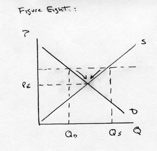
Supply and Demand Interactions.  At last, we consider how prices can be determined through the interaction of supply and demand.   It is simplest to begin with the fiction that suppliers and demanders live in a stable world in which nothing other than the price of their good changes.   Laying supply and demand upon the same graph helps us visualize how buyers and sellers are pushed toward an equilibrium price.   Because buyers and sellers respond oppositely to changes in price, there is only one price that will make their plans the same.  On the graph below, if price is above the equilibrium level—the price at which supply and demand are just equal, then sellers offer more for sale than buyers want.   We can see this more clearly in the Figure 8, in which the Quantity Supplied (Qd) is greater than the Quantity Demanded (Qs).

Figure 7: Equilibrium Pricing

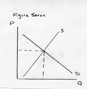
If price is above the equilibrium level, the quantity that sellers (Qs) wish to provide is greater than the quantity that demanders wish to buy (Qd).  In order to unload their goods, sellers may offer their goods for a price somewhat lower.    The expectation is that this leads some sellers to reduce the quantity they supply (a downward movement along their supply curve, which is referred to as a change in the quantity supplied).  However, lower prices would be expected to induce at least some consumers to increase the quantity they demand (moving down to the right along their demand curve).

With these tools you now have sufficient information to anticipate how prices and quantities change when specific variables change.    Before you attempt the problem set, let us review one last major idea.

The idea of equilibrium is central to economics, not because the world comes to rest in equilibrium positions, life is far too dynamic for that, but because equilibrium positions point out the directions for market change.  Most of the time we’ll be happy if we can anticipate changes correctly.  We seldom expect to know exactly what will happen in a world in which so many things depend one upon the other.  So market equilibrium, the place at which supply is just balanced by demand is much like the equilibrium level of water in a mountain lake.  The water level balances the inflow from mountain runoff against the drainages that flow out of the lake at its low points.    Yet, we know that spring flows are apt to be higher and water levels are apt to rise then and fall off in late summer and winter.  But the exact level of the water will keep changing with temperature and precipitation.  Thus, while equilibrium between inflows and outflows generates an equilibrium water level, that water level, like equilibrium prices keeps changing.