Orthogonal Collocation on Finite Elements
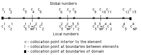
The orthogonal collocation method on finite elements is a useful method for problems whose solution has steep gradients, and the method can be applied to time-dependent problems, too. The method is a bit more complicated than others, since there are combined ordinary differential equations and algebraic equations. The arrangement of collocation points is shown in Figure 1.
Figure 1. Collocation Points for OCFE
Consider the case of diffusion in a slab.

For convenience, all the primes are now dropped.
![]()
The orthogonal collocation on finite elements divides the domain, 0 x 1, into finite elements, and sets the residual to zero at the collocation points interior to the elements. The elements are denoted by the superscript e and the points within an element are denoted by capital I or J. Within the e-th element, we make the transformation
![]()
Then the equations become
![]()
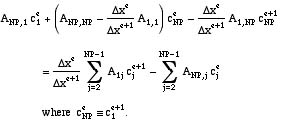
in each element. The orthogonal collocation method is applied at each collocation point interior to the eth-element.
![]()
There are a total of NE*(NP-1)+1 unknowns, where NE is the number of elements and NP is the degree of the polynomial within each element. The above equation gives NE*(NP-2) ordinary differential equations to solve. We need additional conditions. The first of these are presents the condition making the fluxes agree at element edges. Continuity of the function and first derivative between elements requires the condition
![]()
The function is continuous by virtue of assigning it only one value, regardless of whether it is the last point on one element or the first point on the next element. The continuity of first derivative is enforced using
![]()
This provides NE1 conditions. The last two conditions are the boundary conditions.
![]()
Now we have NE*(NP-1)+1 equations. Some of them are algebraic and some of them are ordinary differential equations. Since we are using MATLAB, with an equation solver that assumes all the equations are all ordinary differential equations, we must provide a means to solve the algebraic equations at each point needed by the MATLAB solver.
This is done in the subroutine defining the right-hand side of the ordinary differential equations. One takes the values of the solution at the internal collocation points and solves for the values at the element edges and the boundaries. The continuity of flux at the element edges is satisfied by solving
and the terms on the right-hand side are known. In addition, the two boundary conditions are satisfied by solving
![]()
where again the terms on the right-hand side are known. These NE+1 equations can be solved simultaneously: They form a , which is easily solved. What we have done, essentially, is take the concentration at the points interior to elements, solve this tridiagonal system, and then we have the points at all the collocation points. Then we can evaluate the derivatives at any collocation point simply by knowing what element we are in and using the orthogonal collocation matrices.
The code is available. An illustration is given in Figure 2 for four elements and in Figure 3 for eight elements. Note the fact that the solution is quite good for small time, and is better the more elements are used. This is typical of all numerical methods that use piecewise approximations for this problem. The method of orthogonal collocation on finite elements can be used for small times to better advantage than orthogonal collocation, since the solution is steep and a global polynomial (in orthogonal collocation) requires many terms to approximate the solution. Even so, using only four elements and looking at the solution at t = 0.001 is too severe. Naturally, the smaller closer one gets to a discontinuity, the more (or smaller) elements are necessary.
An example is given for handling boundary conditions more general than those used here.
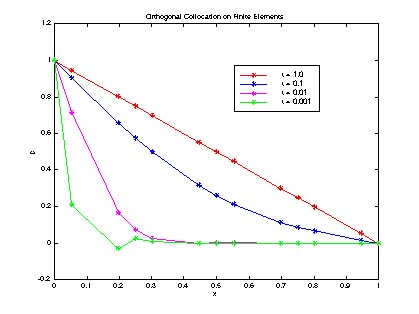
Figure 2. Orthogonal Collocation Solution to Diffusion Problem with 4 Elements
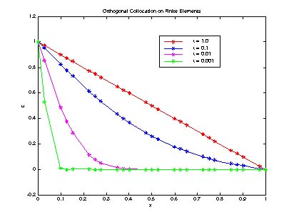
Figure 3. Orthogonal Collocation Solution to Diffusion Problem with 8 Elements
Take Home Message: The method of orthogonal collocation on finite elements is ideally suited to problems involving steep gradients.