Reading: Abel and Bernanke chapter 3, section 1.
Last updated: January 19, 1998.

Introduction to Long-run Supply

The Production Function
Assumptions
Example

Moving Along vs. Shifting Curves
part 1

A Short-run Assumption

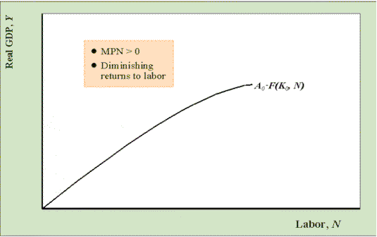
The graph to the right shows the production function as a function of N holding A and K fixed.

The Production Function

The aggregate production function for the economy is assumed to take the form

Y = A·F(K, N)

where

Y = real GDP
A = index of overall productivity in the economy
K = amount of capital input (measured in physical units or in $ value) in the economy
N = number of workers employed in the economy

Assumptions concerning the shape of F(K, N)

Marginal product of labor, MNP, is positive and diminishing

pf1.gif (12955 bytes)

Example: Cobb-Douglas constant returns to scale production function

Y = A·K^aN^1-a , 0 < a < 1

where

a = share of income received by owners of capital
1 - a = share of income received by labor

Note: Constant returns to scale means that if we double all inputs to the productio function then output exactly doubles. To see that the Cobb-Douglas exhibits this property, note that

A·(2K)^a(2N)^1-a = A·2^a2^1-aK^aN^1-a = 2A·K^aN^1-a = 2Y

For US data, from the national income and product accounts, we know that labor's share of income is about 0.7 which implies that for the US a = 0.7 and 1 - a = 0.3.