Reading: AB,
chapter 4.
Last updated on February 19, 1997.
Determining equilibrium in the goods market
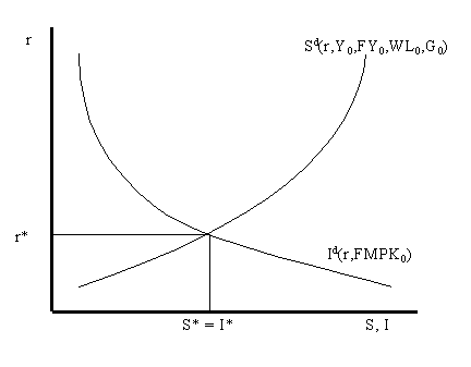
Equilibrium in the market for goods and services occurs when the aggregate demand for goods and services, defined as Yd = Cd + Id + G0, is equal to the aggregate supply of goods and services, Y. Hence in goods market equilibrium Yd = Y =Cd + Id + G0. We may express this goods market equilibrium in a different but equivalent manner. By subtracting Cd +G0 from the left and right hand sides of the equilibrium condition we get: Y - Cd - G0 = Id. Using the fact that, in equilibrium, desired national saving is defined as Sd = Y - Cd - G0 we get the equivalent equilibrium condition: Sd = Id. Therefore, in our economy without a foreign sector we have equilibrium in the market for goods and services if desired national saving is equal to desired investment expenditure. We may represent this equilibrium condition in a savings-investment diagram relating both desired national saving and investment as functions of the real interest rate. This graph is depicted below
In goods market equilibrium the desired savings and investment graphs intersect at the interest rate r* and the desired values of savings and investment are equal and are also equal to the actual values of saving and investment as recorded in the national income and product accounts.
In goods market equilibrium there are no forces acting on savers and investors to move the real interest rate up or down. When the interest rate is such that desired saving is not equal to desired investment then the goods market is not in equilibrium (it is in disequilibrium) and there are market forces acting to move the economy back into equilibrium.
The diagram below illustrates a situation where the real interest rate is higher than the equilibrium interest rate.
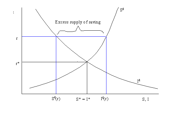
At r > r*, the return to saving is high and the cost of investment is high so that desired saving is greater than desired investment so that there is an excess supply of saving. In this case, banks have more cash on hand than they can loan out to firms. In order to create more loans banks must lower the real interest rate. As r falls, we move down along the savings and investment curves toward the equilibrium point r* where Sd(r*) = Id(r*). A similar analysis corresponds when r < r*.
Increase in current income (Y)
Suppose the goods market is initially in equilibrium with r* =
5% with current income at Y0 as described in the
diagram below. Now suppose that current income (Y), which is
equivalent to current output, increases from Y0 to Y1.
This results in a rightward shift of the desired savings graph as
depicted below.
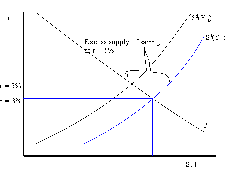
At the real interest rate of 5% there is now an excess supply of saving which puts downward pressure on the real interest rate as banks try to create more loans. As r falls, we move along both the desired saving and investment graphs toward the new equilibrium at r = 3%. The end result of the increase in Y is a lower real interest rate and a higher level of both saving and investment.
Now consider an increase in MPKe due to an increase in business confidence about future profits. This could occur, say, if firms expect that tax laws favoring business may be enacted in the near future. The increase in MPKe leads to a rightward shift up in the desired investment graph holding everything else in the model fixed as illustrated in the graph below.
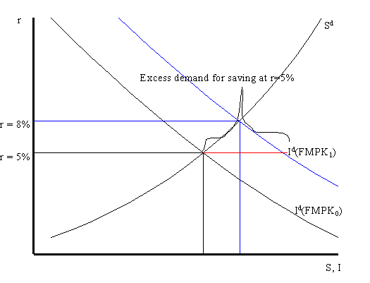
At r = 5%, desired investment is greater than desired saving so that there is an excess demand for saving. Accordingly, banks are able to raise real interest rates due to the increased demand for loans. As r rises, we move up along both the saving and investment graphs toward the new equilibrium at r = 8%.