Econ 301 Lecture 10

Reading: AB, chapter 9 (all) and chapter 11 (all)
Last updated on February 22, 1997.

Introduction to business cycles
Introduction to the classical real business cycle model
Derivation of the aggregate supply and aggregate demand curves

Introduction to the classical real business cycle model

Assumptions

Most markets are competitive.
Prices and wages move quickly to clear markets.
Business cycles are mainly caused by real shocks to the economy.
- Real shock: unexpected change in the production function, labor market or IS curve (saving and investment).
- Nominal shock: unexpected change in money supply or money demand.
Real business cycle theory (RBC) focuses on productivity and government spending shocks as the main sources of business cycles.

Implications of RBC theory

Variable behavior	Consistent with observed data?
Output (Y) is procyclical	Yes
Employment (N) is procyclical	Yes
Avg. labor productivity (Y/N) is procyclical	Yes
Real wage (W/P) is procyclical	Yes - but RBC predicts more variable W/P. The labor supply curve is too steep to be consistent with RBC predictions.
Prices (P) and inflation are counter-cyclical	No - P and inflation appear to be procyclical except for the oil crisis recessions.
Unemployment, u, is always at the natural rate u. Changes in u represent changes in u.	Not really - hard to justify relatively large changes in u.
Monetary policy is neutral	No - money appears to lead the business cycle.
Government spending (G) is procyclical	Yes - if we assume that increases in G make workers poorer.

Policy implications

Fed should not try to stabilize the business cycle - it should only use monetary policy to keep prices stable (inflation under control)
Government need not use fiscal policy (tax and spending policy) to influence aggregate demand to manage the business cycle.
Government should use fiscal policies to stimulate the supply-side of the economy - use policies to promote growth and increase productivity; make labor market more efficient (increase the matching between job seekers and employers).

Derivation of the aggregate supply and aggregate demand curves

Aggregate supply curve

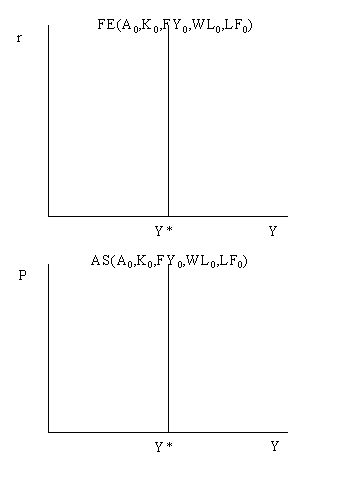
The aggregate supply (AS) curve is derived from the full employment (FE) curve. The AS curve is plotted in a graph with the aggregate price level on the vertical axis and output on the horizontal axis. Recall, the aggregate supply of output is determined by the interaction between the production function and the labor market as summarized by the FE line. In labor market equilibrium, full employment output is Y*. Only changes in the production function or changes in labor demand or labor supply will change Y*. Since the production function and the labor market are not affected by changes in the aggregate price level (it is assumed that any change in P is offset by changes in nominal wages, W, so that the real wage, W/P, stays constant) the aggregate supply curve is a vertical line in the graph with P on the vertical axis and Y on the horizontal axis.

Aggregate demand curve

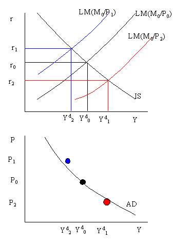
The aggregate demand for goods and services is determined at the intersection of the IS and LM curves independent of the aggregate supply of goods and services (implicitly, when deriving the AD curve it is assumed that whatever is demanded can be supplied by the economy). The AD curve is a plot of the demand for goods as the general price level varies. For a given price level, P₀, the IS and LM curves intersect at the point (r₀, Y^d₀). This intersection point is plotted in the graph below (as the big black dot). If the price level increases to P₁ then the LM curve shift up and left and the new equilibrium is at the point (r₁, Y^d₁). The higher real interest rate has decreased the aggregate demand for goods. This new equilibrium is represented as the big blue dot on the AD curve. Similarly, if the price level drops from P₀ to P₂ then the LM curve shifts down and right lowering the real interest rate and increasing demand. This new equilibrium is given by the big red dot on the AD curve.

The above graphs shows that the AD curve is a downward sloping function of the general price level. This occurs because a low price level (given a fixed money supply) lowers the real interest rate and stimulates interest sensitive demand.