UW STAT 425: Introduction to Nonparametric Statistics (2026 Winter) Lecture 7: Nonparametric Regression

Let $(X_1,Y_1),\cdots,(X_n,Y_n)$ be a bivariate random sample. In the regression analysis, we are often interested in the regression function \[m(x) = \mathbb{E}(Y|X=x).\] Sometimes, we will write \[Y_i = m(X_i) + \epsilon_i,\] where $\epsilon_i$ is a mean $0$ noise. The simple linear regression model is to assume that $m(x) = \beta_0+\beta_1x$, where $\beta_0$ and $\beta_1$ are the intercept and slope parameter. In the first part of the lecture, we will talk about methods that directly estimate the regression function $m(x)$ without imposing any parametric form of $m(x)$. This approach is called the nonparametric regression.

Regressogram (Binning)

We start with a very simple but extremely popular method. This method is called a regressogram, but people often call it the binning approach. You can view it as \[\mbox{regressogram = regression + histogram}.\] For simplicity, we assume that the covariates $X_i$’s are from a distribution over $[0,1]$.

Similar to the histogram, we first choose $M$, the number of bins. Then we partition the interval $[0,1]$ into $M$ equal-width bins: \[B_1=\left[0, \frac{1}{M}\right), B_2=\left[\frac{1}{M}, \frac{2}{M}\right), \cdots, B_{M-1}=\left[\frac{M-2}{M}, \frac{M-1}{M}\right), B_{M}=\left[\frac{M-1}{M}, 1\right].\] When $x\in B_\ell$, we estimate $m(x)$ by \[\widehat{m}_M(x) = \frac{\sum_{i=1}^n Y_i I(X_i\in B_\ell)}{\sum_{i=1}^n I(X_i\in B_\ell)} = \mbox{average of the responses whose covariates are in the same bin as $x$}.\]

Theorem 1. Assume that the PDF of $X$ $p(x)\geq p_0>0$ for all $x\in[0,1]$ and $\mathbb{E}(Y^2|X=x) <\infty$. Then \[{\bf bias}(\widehat{m}_M(x)) = O\left(\frac{1}{M}\right),\quad {\sf Var}(\widehat{m}_M(x)) = O\left(\frac{M}{n}\right).\]

Suppose that $x$ belongs to bin $B_\ell$. Let $\mu_M(x) = \mathbb{E}(Y_iI(X_i\in B_\ell))$ and $q_M(x) = \mathbb{E}(I(X_i\in B_\ell))$ and let $\mu(x) = m(x)\cdot p(x)$.

Using $\widehat m_M(x) = \frac{\widehat\mu_M(x)}{\widehat q_M(x)}$, where \[\widehat\mu_M(x) = \frac{1}{n}\sum_{i=1}^n Y_i I(X_i\in B_\ell), \quad\widehat q_M(x) = \sum_{i=1}^n I(X_i\in B_\ell),\] the difference can be decomposed into \[\widehat m_M(x) - m(x) = \underbrace{\frac{\widehat\mu_M(x)}{\widehat q_M(x)} - \frac{\mu_M(x)}{q_M(x)}}_\text{$\sim$Variance}+\underbrace{\frac{\mu_M(x)}{q_M(x)} - \frac{\mu(x)}{p(x)}}_\text{bias}.\]

Bias. Since we have $M$ bins, the width of each bin is $1/M$. Thus, it is easy to see that $M \cdot q_M(x)$ can be viewed as a density histogram estimator of $p(x)$. Therefore, by the theory of histogram, the bias will be $p(x) - M\cdot q_M(x) = O(1/M)$. Similarly, one can show that $M\cdot\mu_M(x)$ can be viewed as an estimator of $\mu(x)$ and $\mu(x) - M\cdot\mu_M(x) = O(1/M)$. Using the fact that $\frac{1}{1+\epsilon}= 1-\epsilon+O(\epsilon^2)$ when $\epsilon\rightarrow 0$, we conclude that the bias part \[\begin{align*} \frac{\mu_M(x)}{q_M(x)} - \frac{\mu(x)}{p(x)}& = \frac{M\mu_M(x)}{Mq_M(x)} - \frac{\mu(x)}{p(x)}\\ & = \frac{\mu(x)+ O(1/M)}{p(x)+O(1/M)} - \frac{\mu(x)}{p(x)}\\ & = \frac{O(1/M)}{p(x)} + \frac{\mu(x)}{p^2(x)} O(1/M)\\ & = O(1/M). \end{align*}\]

Variance. For the variance part, it is easy to see that $\mathbb{E}(\widehat\mu_M(x)) = \mu_M(x)$ and $\mathbb{E}(\widehat q_M(x)) = q_M(x)$. Also, it is easy to see that the variance (using the same derivation as histogram), \[{\sf Var}(\widehat\mu_M(x)) = O\left(\frac{1}{Mn}\right), \quad {\sf Var}(\widehat q_M(x)) = O\left(\frac{1}{Mn}\right).\] Thus, \[{\sf Var}(M\widehat\mu_M(x)) = O\left(\frac{M}{n}\right),\quad {\sf Var}(M\widehat q_M(x)) = O\left(\frac{M}{n}\right).\] Let $\Delta_\mu(x) = M\widehat\mu_M(x) - M \mu_M(x) = O_P(\sqrt{M/n})$ and $\Delta_q(x) = M\widehat q_M(x) - Mq_M(x)= O_P(\sqrt{M/n})$. Then \[\begin{align*} \frac{\widehat\mu_M(x)}{\widehat q_M(x)} - \frac{\mu_M(x)}{q_M(x)} & = \frac{M\widehat\mu_M(x)}{M\widehat q_M(x)} - \frac{M\mu_M(x)}{Mq_M(x)}\\ & = \frac{M \mu_M(x) + \Delta_\mu(x) }{ Mq_M(x) + \Delta_q(x) } - \frac{M\mu_M(x)}{Mq_M(x)}\\ & = \frac{M\mu_M(x) +\Delta_\mu(x)}{Mq_M(x)} - \frac{M\mu_M(x)}{M^2q_M^2(x)} \Delta_q(x) - \frac{M\mu_M(x)}{Mq_M(x)} + \mbox{ smaller order terms}\\ & \approx \frac{1}{Mq_M(x)} \Delta_\mu(x) - \frac{M\mu_M(x)}{M^2q_M^2(x)} \Delta_q(x)\\ & \approx \frac{1}{p(x)} \Delta_\mu(x) - \frac{\mu(x)}{p^2(x)} \Delta_q(x). \end{align*}\] Note that the last $\approx$ sign is due to the bias analysis. Thus, the variance of $\frac{\widehat\mu_M(x)}{\widehat q_M(x)}$ equals the variance of $\frac{1}{p(x)} \Delta_\mu(x) - \frac{\mu(x)}{p^2(x)} \Delta_q(x)$, which is of rate $O(M/n)$.

Therefore, the MSE and MISE will be at rate \[{\bf MSE} = O\left(\frac{1}{M^2}\right) +O\left(\frac{M}{n}\right),\quad {\bf MISE} = O\left(\frac{1}{M^2}\right) +O\left(\frac{M}{n}\right),\] leading to the optimal number of bins $M^*\asymp n^{1/3}$ and the optimal convergence rate $O(n^{-2/3})$, the same as the histogram.

Similar to the histogram, the regressogram has a slower convergence rate compared to many other competitors (we will introduce several other candidates). However, they (histogram and regressogram) are still very popular because the construction of an estimator is very simple and intuitive; practitioners with little mathematical training can easily master these approaches.

Note that if we assume that the response variable $Y$ is bounded, you can construct a similar concentration bound as the case of histogram and obtain the rate under the $L_\infty$ metric.

Kernel Regression

Given a point $x_0$, assume that we are interested in the value $m(x_0)$. Here is a simple method to estimate that value. When $m(x_0)$ is smooth, an observation $X_i\approx x_0$ implies $m(X_i)\approx m(x_0)$. Thus, the response value $Y_i = m(X_i)+\epsilon_i\approx m(x_0)+\epsilon_i$. Using this observation, to reduce the noise $\epsilon_i$, we can use the sample average. Thus, an estimator of $m(x_0)$ is to take the average of those responses whose covariates are close to $x_0$.

To make it more concrete, let $h>0$ be a threshold. The above procedure suggests using \[\begin{equation} \widehat{m}_{\sf loc}(x_0) = \frac{\sum_{i: |X_i-x_0|\leq h}Y_i}{n_h(x_0)} = \frac{\sum_{i=1}^n Y_iI(|X_i-x_0|\leq h)}{\sum_{i=1}^n I(|X_i-x_0|\leq h)}, \label{eq::loc} \end{equation}\] where $n_h(x_0)$ is the number of observations where the covariate $X:|X_i-x_0|\leq h$. This estimator, $\widehat{m}_{\sf loc}$, is called the local average estimator. Indeed, to estimate $m(x)$ at any given point $x$, we are using a local average as an estimator.

The local average estimator can be rewritten as \[\begin{equation} \widehat{m}_{\sf loc}(x_0) = \frac{\sum_{i=1}^n Y_iI(|X_i-x_0|\leq h)}{\sum_{i=1}^n I(|X_i-x_0|\leq h)} = \sum_{i=1}^n\frac{I(|X_i-x_0|\leq h)}{\sum_{\ell=1}^n I(|X_\ell-x_0|\leq h)}\cdot Y_i = \sum_{i=1}^n W_i(x_0) Y_i, \label{eq::wloc} \end{equation}\] where \[\begin{equation} W_i(x_0) = \frac{I(|X_i-x_0|\leq h)}{\sum_{\ell=1}^n I(|X_\ell-x_0|\leq h)} \label{eq::weight} \end{equation}\] is a weight for each observation. Note that $\sum_{i=1}^n W_i(x_0) = 1$ and $W_i(x_0)>0$ for all $i=1,\cdots,n$; this implies that $W_i(x_0)$’s are indeed weights. Equation $\eqref{eq::wloc}$ shows that the local average estimator can be written as a weighted average estimator so the $i$-th weight $W_i(x_0)$ determines the contribution of response $Y_i$ to the estimator $\widehat{m}_{\sf loc}(x_0)$.

In constructing the local average estimator, we are placing a hard-thresholding on the neighboring points–those within a distance $h$ are given equal weight but those outside the threshold $h$ will be ignored completely. This hard-thresholding leads to an estimator that is not continuous.

To avoid this problem, we consider another construction of the weights. Ideally, we want to give more weights to those observations that are close to $x_0$ and we want to have a weight that is ‘smooth’. The Gaussian function $G(x) = \frac{1}{\sqrt{2\pi}}e^{-x^2/2}$ seems to be a good candidate. We now use the Gaussian function to construct an estimator. We first construct the weight \[W^G_i(x_0 ) = \frac{G\left(\frac{x_0-X_i}{h}\right)}{\sum_{\ell=1}^n G\left(\frac{x_0-X_\ell}{h}\right)}.\] The quantity $h>0$ is a similar quantity to the threshold in the local average but now it acts as the smoothing bandwidth of the Gaussian. After constructing the weight, our new estimator is \[\begin{equation} \widehat{m}_{\sf G}(x_0) = \sum_{i=1}^n W^G_i(x_0 ) Y_i = \sum_{i=1}^n \frac{G\left(\frac{x_0-X_i}{h}\right)}{\sum_{\ell=1}^n G\left(\frac{x_0-X_\ell}{h}\right)}Y_i =\frac{\sum_{i=1}^n Y_i G\left(\frac{x_0-X_i}{h}\right)}{\sum_{\ell=1}^n G\left(\frac{x_0-X_\ell}{h}\right)}. \label{eq::Gaussian} \end{equation}\] This new estimator has a weight that changes more smoothly than the local average and is smooth as we desire.

Observing from equation $\eqref{eq::loc}$ and $\eqref{eq::Gaussian}$, one may notice that these local estimators are all of a similar form: \[\begin{equation} \widehat{m}_h(x_0) =\frac{\sum_{i=1}^n Y_i K\left(\frac{x_0-X_i}{h}\right)}{\sum_{\ell=1}^n K\left(\frac{x_0-X_\ell}{h}\right)}= \sum_{i=1}^n W^K_i(x_0 ) Y_i , \quad W^K_i(x_0 ) =\frac{K\left(\frac{x_0-X_i}{h}\right)}{\sum_{\ell=1}^n K\left(\frac{x_0-X_\ell}{h}\right)}, \label{eq::kernel} \end{equation}\] where $K$ is some function. When $K$ is a Gaussian, we obtain estimator $\eqref{eq::Gaussian}$; when $K$ is a uniform over $[-1,1]$, we obtain the local average $\eqref{eq::loc}$. The estimator in equation $\eqref{eq::kernel}$ is called the kernel regression estimator or Nadaraya-Watson estimator¹. The function $K$ plays a similar role as the kernel function in the KDE and thus it is also called the kernel function. And the quantity $h>0$ is similar to the smoothing bandwidth in the KDE so it is also called the smoothing bandwidth.

Plug-in estimator perspective

The kernel regression can be viewed as a plug-in estimator from a multivariate KDE. Since the regression function \[m(x) = \mathbb{E}(Y|X=x) = \int y p(y|x)dy,\] a plug-in estimator of $m(x)$ is via \[\widehat m(x) = \int y \widehat p(y|x)dy,\] where $\widehat p(y|x)$ is an estimator of the conditional PDF. The plug-in approach essentially implies that we can convert a multivariate density estimator into a regression estimator. Moreover, if our plug-in estimator is a KDE with product kernel, the regression estimator is the kernel regression.

In more detail, using the given bivariate random sample $(X_1,Y_1), \cdots, (X_n,Y_n)$, we can estimate the joint PDF $p(x,y)$ as \[\widehat{p}_n(x,y) = \frac{1}{nh^2} \sum_{i=1}^n K\left(\frac{X_i-x}{h}\right)K\left(\frac{Y_i-y}{h}\right).\] This joint density estimator also leads to a marginal density estimator of $X$: \[\widehat{p}_n(x) = \int \widehat{p}_n(x,y)dy = \frac{1}{nh}\sum_{i=1}^n K\left(\frac{X_i-x}{h}\right).\]

Theorem 2. The conditional expectation of $Y$ given $X=x$ implied by the $2D$ KDE is the same as the kernel regression estimator.

Recall that the regression function is the conditional expectation \[m(x) = \mathbb{E}(Y|X=x) = \int yp(y|x)dy = \int y \frac{p(x,y)}{p(x)}dy = \frac{\int y p(x,y)dy}{p(x)}.\] Replacing $p(x,y)$ and $p(x)$ by their corresponding estimators $\widehat{p}_n(x,y)$ and $\widehat{p}_n(x)$, we obtain an estimate of $m(x)$ as \[\begin{align*} \widehat{m}_n(x) &=\frac{\int y \widehat{p}_n(x,y)dy}{\widehat{p}_n(x)} \\ &= \frac{\int y \frac{1}{nh^2} \sum_{i=1}^n K\left(\frac{X_i-x}{h}\right)K\left(\frac{Y_i-y}{h}\right)dy}{\frac{1}{nh}\sum_{i=1}^n K\left(\frac{X_i-x}{h}\right)}\\ & = \frac{\sum_{i=1}^nK\left(\frac{X_i-x}{h}\right) \cdot \int y\cdot K\left(\frac{Y_i-y}{h}\right)\frac{dy}{h}}{\sum_{i=1}^n K\left(\frac{X_i-x}{h}\right)}\\ & = \frac{\sum_{i=1}^nK\left(\frac{X_i-x}{h}\right) Y_i}{\sum_{i=1}^n K\left(\frac{X_i-x}{h}\right)}\\ & = \frac{\sum_{i=1}^nY_iK\left(\frac{X_i-x}{h}\right) }{\sum_{i=1}^n K\left(\frac{X_i-x}{h}\right)}\\ & = \widehat{m}_h(x). \end{align*}\] Note that when $K(x)$ is symmetric, $\int y\cdot K\left(\frac{Y_i-y}{h}\right)\frac{dy}{h} = Y_i$.

Namely, we may understand the kernel regression as an estimator inverting the KDE of the joint PDF into a regression estimator.

Local least square perspective

The kernel regression can be viewed as a local least squares estimator. To see this, recall that the mean of a random variable $Y$ can be written as \[\mathbb{E}(Y) = {\sf argmin}_c\quad \mathbb{E}((Y-c)^2).\] Thus, the conditional mean satisfies \[\mathbb{E}(Y|X=x) = {\sf argmin}_c\quad \mathbb{E}(I(X=x)(Y-c)^2).\] When $X$ is discrete, we can replace the expectation with sample average, leading to \[\widehat{\mathbb{E}}(Y|X=x) = {\sf argmin}_c\quad \frac{1}{n}\sum_{i=1}^n I(X_i=x) (Y_i-c)^2.\]

However, if $X$ is continuous, the indicator function $I(X_i=x)$ is almost always $0$. To resolve this problem, we can consider relaxing $I(X_i=x) = I(\|X_i-x\|_2 = 0)$ into \[I(X=x) = I(\|X-x\|_2 = 0)\approx I(\|X-x\|_2 \leq h) = I\left(\frac{\|X-x\|_2}{h}\leq 1\right) \approx K\left(\frac{X-x}{h}\right).\] This kernelization method relaxes the indicator function into a kernel function centered at $x$.

Note that when $x$ is multivariate, the kernel function will be a multivariate kernel. With the above relaxation, we can easily see that \[\begin{equation} \mathbb{E}(Y|X=x) = {\sf argmin}_c\quad \mathbb{E}(I(X=x)(Y-c)^2) \approx {\sf argmin}_c\quad \mathbb{E}\left(K\left(\frac{X-x}{h}\right)(Y-c)^2\right). \label{eq::localLS} \end{equation}\] The relaxed objective function $R_h(c) = \mathbb{E}\left(K\left(\frac{X-x}{h}\right)(Y-c)^2\right)$ can be estimated easily via \[\widehat R_h(c ) = \frac{1}{n}\sum_{i=1}^n K\left(\frac{X_i-x}{h}\right)(Y_i-c)^2\] and the minimizer \[\widehat c_h = \frac{\sum_{i=1}^n Y_i K\left(\frac{X_i-x}{h}\right)}{\sum_{i'=1}^n K\left(\frac{X_{i'}-x}{h}\right)} = \widehat m_h(x)\] is the kernel regression estimator.

Note that kernelization is not the only approach to relax the indicator function $I(X=x)$. We can use other localization methods such as k-nearest neighbor (kNN). In this case, we relax \[I(X=x) \approx I(X \in N_k(x)),\] where $N_k(x)$ is the $k$-nearest neighborhood at $x$. Namely, \[N_k(x) = B(x, R_k(x)),\qquad R_k(x) = \min\left\{r>0: \sum_{i=1}^n I(\|X_i-x\|_2 \leq r)\geq k \right\},\] where $R_k(x)$ is the distance from $x$ to the $k$-th nearest observation. If we use the kNN relaxation $I(X=x) \approx I(X \in N_k(x))$, the resulting estimator is the kNN regression.

Theory

Now we study some statistical properties of the estimator $\widehat{m}_h$. Suppose that we are interested in $m(x)$ over a compact interval $\mathbb{K}\subset \mathbb{R}$.

Theorem 3. Assume that

$\inf_{x\in \mathbb{K}}p(x)>0$ and $p(x)$ has bounded second derivatives.
$\mathbb{E}(Y^2|X=x)<\infty$ and $m(x)$ has bounded third derivatives.

Then \[\begin{align*} {\bf bias}(\widehat{m}_h(x)) &= \frac{h^2}{2} \mu_K \left(m''(x)+2\frac{m'(x)p'(x)}{p(x)}\right) + o(h^2)\\ {\sf Var}(\widehat{m}_h(x)) &= \frac{\sigma^2 \cdot \sigma_K^2}{p(x)}\cdot \frac{1}{nh} +o\left(\frac{1}{nh}\right), \end{align*}\] where $\mu_K = \int x^2 K(x)dx$ is the same constant of the kernel function as in the KDE and $\sigma^2 = {\sf Var}(\epsilon_i)$ is the error of the regression model and $\sigma_K^2 = \int K^2(x)dx$ is a constant of the kernel function (the same as in the KDE).

The bias has two components: a curvature component $m''(x)$ and a design component $\frac{m'(x)p'(x)}{p(x)}$. The curvature component is similar to the one in the KDE; when the regression function curved a lot, kernel smoothing will smooth out the structure, introducing some bias. The second component, also known as the design bias, is a new component compare to the bias in the KDE. This component depends on the density of covariate $p(x)$. Note that in some studies, we can choose the values of covariates so the density $p(x)$ is also called the design (this is why it is known as the design bias).

The expression of variance tells us possible sources of variability. First, the variance increases when $\sigma^2$ increases. This makes perfect sense because $\sigma^2$ is the noise level. When the noise level is large, we expect the estimation error increases. Second, the density of covariate $p(x)$ is inversely related to the variance. This is also very reasonable because when $p(x)$ is large, there tends to be more data points around $x$, increasing the size of sample that we are averaging from. Last, the convergence rate is $O\left(\frac{1}{nh}\right)$, which is the same as the KDE.

MSE and MISE. Using the expression of bias and variance, the MSE at point $x$ is \[{\bf MSE}(\widehat{m}_h(x)) = \frac{h^4}{4} \mu_K^2 \left(m''(x)+2\frac{m'(x)p'(x)}{p(x)}\right)^2 + \frac{\sigma^2 \cdot \sigma_K^2}{p(x)}\cdot \frac{1}{nh}+o(h^4) +o\left(\frac{1}{nh}\right)\] and the MISE is \[\begin{equation} {\bf MISE}(\widehat{m}_h) %= \int {\bf MSE}(\hat{m}_h(x))dx = \frac{h^4}{4} \mu_K^2 \int\left(m''(x)+2\frac{m'(x)p'(x)}{p(x)}\right)^2dx + \frac{\sigma^2 \cdot \sigma_K^2}{nh}\int\frac{1}{p(x)}dx+o(h^4) +o\left(\frac{1}{nh}\right). \label{eq::MISE} \end{equation}\] Optimizing the major components in equation $\eqref{eq::MISE}$ (the AMISE), we obtain the optimal value of the smoothing bandwidth \[h_{\sf opt} = C^* \cdot n^{-1/5},\] where $C^*$ is a constant depending on $p$ and $K$.

Cross-Validation

In nonparametric regression, we often have a tuning parameter such as the smoothing bandwidth $h$ for kernel regression or the number of bins $M$ for regressogram. We need to choose these tuning parameters before constructing our estimator.

While our bias-variance analysis offers us an insight into the optimal tuning parameter such as $h_{\sf opt} = C^* \cdot n^{-1/5}$ for the kernel regression, this involves an unknown quantity $C^*$. So in practice, how can we choose it? A good news is that–unlike the density estimation problem, there is a simple approach to choose $h$ (or $M$ for regressogram or other tuning parameters): the cross-validation (CV)².

Before we discuss the details of CV, we first introduce the predictive risk. Let $\widehat{m}_h$ be the kernel regression using the $n$ observations. Let $X_{n+1},Y_{n+1}$ be a new observation (from the same population). We define the predictive risk of our regression estimator as \[\begin{equation} R(h) = \mathbb{E}\left(Y_{n+1} - \widehat{m}_h(X_{n+1})\right)^2. \end{equation}\] Namely, the quantity $R(h)$ is the expected square error of predicting the next observation using the kernel regression.

CV is a collection of approaches that tries to estimate the predictive risk $R(h)$ using a data-splitting approach. A classical version of CV is the leave-one out cross-validation (LOO-CV): \[\widehat{R}(h) = \frac{1}{n}\sum_{i=1}^n (Y_i-\widehat{m}_{h,-i}(X_i))^2,\] where $\widehat{m}_{h,-i}(X_i)$ is the kernel regression using all observations except $i$-th observation $X_i,Y_i$. Namely, LOO-CV leaves each observation out once at a time and use the remaining observations to train the estimator and evaluate the quality of the estimator using the left out observation. The main reasoning of such a procedure is to make sure we do not use the data twice.

Another popular version of CV is the K-fold CV. We randomly split the data into K equal size groups. Each time we leave out one group and use the other K-1 groups to construct our estimator. Then we use the left out group to evaluate the risk. Repeat this procedure many times and take the average as the risk estimator $\widehat{R}(h)$.

The CV provides a simple approach of estimating the predictive errors. To choose the smoothing bandwidth, we pick \[h^* = {\sf argmin}_{h>0} \widehat{R}(h).\] In practice, we apply the CV to various values of $h$ and choose the one with the minimal predictive risk. Generally, we will plot $\widehat{R}(h)$ versus $h$ and determine if the minimal value makes sense. Sometimes there might be no well-defined minimum value (like a flat region).

Why do we want to split the data into two parts and construct the estimator on one part and evaluate the risk on the other part? The main reason is to obtain a reliable estimate of the predictive risk. If we use the same set of data to construct our estimator and evaluate the errors, the estimated predictive risk will be smaller than the actual predictive risk. To see this, consider the local average estimator with $h\approx 0$. When $h$ is very very small, $\widehat{m}_{\sf loc}(X_i) = Y_i$ because the neighborhood only contain this single observation. In this case, the estimated predictive risk will be $\sum_{i=1}^n(Y_i-Y_i)^2 = 0$. This is related to the so-called overfitting³.

The cross-validation is a very popular and common approach to choose a tuning parameter. Other tuning parameters such as the number of basis $N$ and the penalization $\lambda$ (will be introduced in a minute) can all be chosen by minimizing the cross-validation error.

Local Polynomial Regression (Optional)

The kernel regression estimator has a limitation that it suffers a lot from the boundary bias, i.e., when $x$ is close to the support of $p(x)$, the bias will be very large. To address this issue, we may use a modified estimator called the local polynomial regression (LPR).

LPR starts with the following localized least squares estimation problem. Suppose that we want to estimate the regression function $m(x)$ at point $x$. Consider fitting the following local linear function \[{\sf LPR}(\beta_0,\beta_1;x) = \sum_{i=1}^n K\left(\frac{x-X_i}{h}\right) (Y_i-\beta_0-\beta_1(X_i-x))^2,\] where $K(\cdot)$ is the usual kernel function. This is fitting a weighted linear regression where the observations close to $x$ are given higher weights. The above local linear criterion can be viewed as a generalization of equation $\eqref{eq::localLS}$ that we allow a linear term. Let $\widehat\beta_0(x),\widehat\beta_1(x)$ be the minimizer of ${\sf LPR}(\beta_0,\beta_1;x)$. Then the estimator $\widehat\beta_0(x)$ is called the local linear smoother and is a consistent estimator of $m(x)$, the regression function.

There is a closed-form of the local linear smoother. Define the diagonal matrix \[W(x)\in\mathbb{R}^{n\times n} = {\sf Diag}\left(K\left(\frac{x-X_1}{h}\right),\cdots, K\left(\frac{x-X_n}{h}\right)\right)\] and the matrix $\mathbb{X}\in\mathbb{R}^{n\times 2}$ \[\mathbb{X} = ( 1_n,X-x1_n),\] where $X$ is a column vector of $X_1,\cdots, X_n$ and $1_n$ is a column vector of $1$’s. Let $\mathbb{Y}$ be the column vector of $Y_1,\cdots, Y_n$. Using the derivation as linear regression, you can show that the local linear smoother $\widehat\beta_0(x)$ is \[\widehat\beta_0(x) = e_1^T(\mathbb{X}^TW(x)\mathbb{X})^{-1} \mathbb{X}^TW(x)\mathbb{Y} ,\] where $e_1^T = (1,0)$ is a $1\times 2$ vector. We write $\widehat m_{\sf LL}(x) = \widehat\beta_0(x)$.

We can generalize the local linear smoother to higher order polynomials. For instance, we can fit it to the $q$-th order polynomial \[{\sf LPR}(\beta_0,\beta_1,\cdots, \beta_q;x) = \sum_{i=1}^n K\left(\frac{x-X_i}{h}\right) (Y_i-\beta_0-\beta_1(X_i-x)-\cdots \beta_q(X_i-x)^q)^2.\] Fitting a higher order polynomial is often used to estimate the derivative of the regression function. In fact, if we want to consistently estimate $m^{(\beta)}$, the $\beta-$the derivative of $m(x)$, then we will fit a $(\beta+1)$-th order polynomial. Using the same derivation as the local linear smoother, you can obtain a closed-form of the estimator.

Theorem 4 (Fan (1992)). Suppose that $Y_i = m(X_i)+\sigma(X_i)\epsilon_i$ and $X_i \in\mathbb{K}$ with $\mathbb{E}(\epsilon_i) =0,{\sf Var}(\epsilon_i)=1$ and $X_1,\cdots, X_n\sim p$ and we are interested in a point $x$ in the interior of $\mathbb{K}$. Assume the following:

$p(x)>0$.
$p$, $m''$, and $\sigma$ are continuous in the neighborhood of $x$.
$h\rightarrow0$, $nh\rightarrow\infty$.

Then the local linear smoother satisfies \[{\bf bias}(\widehat m_{\sf LL}(x)) = \frac{h^2}{2}m''(x)\mu_K + o(h^2),\quad {\sf Var}(\widehat m_{\sf LL}(x)) =\frac{\sigma^2(x)}{p(x)nh} \sigma^2_K + o\left(\frac{1}{nh}\right).\]

Namely, the local linear smoother does not suffer from the design bias. The above theorem is from the following paper:

Linear Smoother

Now we are going to introduce a very important notion called a linear smoother. A linear smoother is a collection of many regression estimators that have nice properties. A linear smoother is an estimator of the regression function in the form that \[\begin{equation} \widehat{m}(x) = \sum_{i=1}^n \ell_i(x) Y_i, \end{equation}\] where $\ell_i(x)$ is some function depending on $X_1,\cdots,X_n$ but not on any of $Y_1,\cdots, Y_n$.

The residual for the $j$-th observation can be written as \[e_j = Y_j-\widehat{m}(X_j) = Y_j-\sum_{i=1}^n \ell_i(X_j) Y_i.\] Let $e = (e_1,\cdots,e_n)^T$ be the vector of residuals and define an $n\times n$ matrix $L$ as $L_{ij} = \ell_j(X_i)$: \[L = \begin{pmatrix} \ell_1(X_1)&\ell_2(X_1)&\ell_3(X_1)&\cdots &\ell_n(X_1)\\ \ell_1(X_2)&\ell_2(X_2)&\ell_3(X_2)&\cdots &\ell_n(X_2)\\ \vdots&\vdots&\vdots&\vdots& \vdots\\ \ell_1(X_n)&\ell_2(X_n)&\ell_3(X_n)&\cdots &\ell_n(X_n)\\ \end{pmatrix}\] Then the predicted vector $\widehat{\mathbb{Y}} = (\widehat{Y}_1,\cdots, \widehat{Y}_n)^T = LY$, where $\mathbb{Y} = (Y_1,\cdots,Y_n)^T$ is the vector of observed $Y_i$’s and $e = \mathbb{Y}-\widehat{\mathbb{Y}}= \mathbb{Y}-L\mathbb{Y} = (I-L)\mathbb{Y}$.

Example: Linear Regression. For the linear regression, let $\mathbb{X}$ denote the data matrix (first column is all values $1$ and second column is $X_1,\cdots,X_n$). We know that $\widehat{\beta} = (\mathbb{X}^T\mathbb{X})^{-1}\mathbb{X}^T\mathbb{Y}$ and $\widehat{\mathbb{Y}} = \mathbb{X}\widehat{\beta} = \mathbb{X}(\mathbb{X}^T\mathbb{X})^{-1}\mathbb{X}^T \mathbb{Y}$. This implies that the matrix $L$ is \[L = \mathbb{X}(\mathbb{X}^T\mathbb{X})^{-1}\mathbb{X}^T,\] which is also the projection matrix in linear regression. Thus, the linear regression is a linear smoother.

Example: Regressogram. The regressogram is also a linear smoother. Let $B_1,\cdots,B_m$ be the bins of the covariate and define $B(x)$ to be the bin such that $x$ belongs to it. Then \[\ell_j(x) = \frac{I(X_j\in B(x))}{\sum_{i=1}^nI(X_i\in B(x))}.\]

Example: Kernel Regression. As you may expect, the kernel regression is also a linear smoother. Recall from equation $\eqref{eq::kernel}$ \[\widehat{m}_h(x_0) =\frac{\sum_{i=1}^n Y_i K\left(\frac{x_0-X_i}{h}\right)}{\sum_{\ell=1}^n K\left(\frac{x_0-X_\ell}{h}\right)}= \sum_{i=1}^n W^K_i(x_0 ) Y_i , \quad W^K_i(x_0 ) =\frac{K\left(\frac{x_0-X_i}{h}\right)}{\sum_{\ell=1}^n K\left(\frac{x_0-X_\ell}{h}\right)}\] so \[\ell_j(x) = \frac{K\left(\frac{x-X_j}{h}\right)}{\sum_{\ell=1}^n K\left(\frac{x-X_\ell}{h}\right)}.\]

Example: Local Linear Smoother. You can easily show that the LPR is a linear smoother. In particular, the linear smoother has the vector $\ell(x) = (\ell_1(x),\cdots,\ell_n(x))^T$ as \[\ell(x) = e_1^T(\mathbb{X}^TW(x)\mathbb{X})^{-1} \mathbb{X}^TW(x).\]

Variance of Linear Smoother

The linear smoother has an unbiased estimator of the underlying noise level $\sigma^2$ under the fixed design, i.e., the covariates are non-random. Recall that the noise level $\sigma^2 = {\sf Var}(\epsilon_i)$.

We need to use two tricks about variance and covariance matrix. For a matrix $A$ and a random variable $X$, \[{\sf Cov}(AX) = A{\sf Cov}(X) A^T.\] Thus, the covariance matrix of the residual vector \[\begin{align*} {\sf Cov}(e) = {\sf Cov} ((I-L)\mathbb{Y}) = (I-L){\sf Cov}(\mathbb{Y})(I-L^T). \end{align*}\] Because $Y_1,\cdots, Y_n$ are IID, ${\sf Cov}(\mathbb{Y}) = \sigma^2 \mathbb{I}_n$, where $\mathbb{I}_n$ is the $n\times n$ identity matrix. This implies \[{\sf Cov}(e) = (I-L){\sf Cov}(\mathbb{Y})(I-L^T) = \sigma^2 (I-L-L^T +LL^T).\]

Now taking matrix trace on both sides, \[{\sf Tr} ({\sf Cov}(e)) = \sum_{i=1}^n {\sf Var}(e_i) = \sigma^2{\sf Tr}(I-L-L^T +LL^T) = \sigma^2 (n-\nu-\nu+\widetilde{\nu}),\] where $\nu= {\sf Tr}(L)$ and $\widetilde{\nu} = {\sf Tr}(LL^T)$. Because the residual square is approximately ${\sf Var}(e_i)$, we have \[\sum_{i=1}^n e_i^2 \approx \sum_{i=1}^n {\sf Var}(e_i) = \sigma^2 (n-2\nu+\widetilde{\nu}).\] Thus, we can estimate $\sigma^2$ by \[\begin{equation} \widehat{\sigma}^2 = \frac{1}{n-2\nu+\widetilde{\nu}} \sum_{i=1}^n e_i^2. \label{eq::var_est} \end{equation}\] The quantity $\nu$ is called the degrees of freedom. In the linear regression case, $\nu = \widetilde{\nu} = p+1$, the number of covariates so the variance estimator $\widehat{\sigma}^2 = \frac{1}{n-p-1} \sum_{i=1}^n e_i^2$. If you have learned the variance estimator of a linear regression, you should be familiar with this estimator.

The degrees of freedom $\nu$ is easy to interpret in the linear regression. And the power of equation $\eqref{eq::var_est}$ is that it works for every linear smoother as long as the errors $\epsilon_i$’s are IID. So it shows how we can define effective degrees of freedom for other complicated regression estimator.

Basis regression

The basis approach is widely used in modern machine learning (ML) and artificial intelligence (AI). The basis functions could be either a given set of functions (such as polynomial functions, or spline functions with fixed knots) or learned from data (data-driven). Let \[\{\phi_1(x),\phi_2(x),\phi_3(x),\cdots \}\] be a collection of basis functions (linearly independent from each other).

As you can see, there are many data-driven methods for finding a basis function. The problem learning basis functions is a central topic in representation learning (also known as feature learning).

When using basis regression, we attempt to approximate $m(x) = \mathbb{E}(Y|X=x)$ by \[m(x) \approx \sum_{j=1} \theta_j\phi_j(x)\] and we estimate $\theta_j$ using the least square method.

Suppose we have $M$ basis functions, we are approximating \[Y_i\approx \sum_{j=1}^M \theta_j \phi_j(X_i).\] With this, we estimate $\theta$ by \[\begin{equation} \widehat\theta_{LS} = {\sf argmin}_\theta \quad \frac{1}{n}\sum_{i=1}^n \left(Y_i - \sum_{j=1}^M \theta_j \phi_j(X_i)\right)^2. \label{eq::LM} \end{equation}\]

You may have noticed that the above form looks like linear regression. Indeed, it can be written as a linear model. Let $\theta = (\theta_1,\cdots,\theta_M)^T$ be the parameter vector and $\Phi \in \mathbb{R}^{n\times M}$ be the ‘design’ matrix such that \[\Phi_{ij} = \phi_j(X_i)\] and $\mathbb{Y} = (Y_1,\cdots, Y_n)^T$. Then the least square estimator in equation $\eqref{eq::LM}$ can be written as \[\begin{equation} \widehat\theta_{LS} = {\sf argmin}_\theta \quad \frac{1}{n}\|\mathbb{Y} - \Phi \theta\|^2_2, \label{eq::LM2} \end{equation}\] which leads to a closed-form solution \[\widehat\theta_{LS} = (\Phi^T\Phi)^{-1}\Phi^T \mathbb{Y}.\]

Under the least square method with $M$ basis coefficients, there are effectively $M$ parameters. Thus, we do need $M$ to be smaller than the sample size but this is a condition that is easily satisfied.

The least square approach has a benefit that you can easily combine it with penalization method (adding $L_1$ or $L_2$ penalization) because it is essentially a linear model problem. This is particularly useful when there are more than one covariate.

Note: you can easily see that all of the above basis regression methods are linear smoother–the matrix $(\Phi^T\Phi)^{-1}\Phi^T$ does not depend on any outcome variable $Y$.

Neural nets

The conventional neural networks for regression may be viewed as a basis regression approach. However, they differ from traditional basis regression methods in the sense that the basis in a neural net is learned using information from the outcome variable $Y$.

To see this, we consider a very simple ReLU (Rectified Linear Unit) neural net. Namely, we choose the activation function to be $\max\{0,x\}$. Consider the ReLU function $\sigma(z) = \max\{0,z\}$. For a vector ${z} \in \mathbb{R}^d$, we define the element-wise activation $\sigma_d: \mathbb{R}^d \to \mathbb{R}^d$ such that $(\sigma_d({z}))_j = \sigma(z_j) = \max\{0, z_j\}$ for $j=1,\cdots, d$. Suppose our data consists of IID random elements \[(X_1,Y_1),\cdots, (X_n,Y_n) \in \mathbb{R}^{d_1}\times \mathbb{R}\] Then we define the function $G_\theta: \mathbb{R}^{d_1} \to\mathbb{R}^{d_3}$ \[G_\theta(x) = \sigma_{d_3} (W_2 \sigma_{d_2}(W_1x+b_1)+b_2),\] where $W_1\in \mathbb{R}^{d_2\times d_1}, W_2 \in \mathbb{R}^{d_3\times d_2}, b_1\in\mathbb{R}^{d_2}, b_2 \in \mathbb{R}^{d_3}$ are the parameters in the neural net. $G_\theta$ is a two-layer ReLU neural net that is parametrized by $\theta = (W_1,W_2,b_1,b_2)$. Suppose $\theta$ is given, our final prediction model is to find $\beta\in\mathbb{R}^{d_3}, \alpha\in\mathbb{R}$ that minimizes \[\min_{\beta,\alpha}\quad \sum_{i=1}^n (Y_i - \beta^TG_\theta(X_i)-\alpha)^2.\] Thus, this can be viewed as a basis approach with the basis function \[\{\phi_0(x) \equiv 1, \phi_1(x),\cdots, \phi_{d_3}(x)\}\] such that $\phi_j(x) = G_{\theta, j}(x)$, the $j$-th element of $G_\theta(x)$ for $j=1,2,\cdots, d_3$.

However, a crucial difference between neural nets and other basis regression is that we estimate/learn $\theta$ using the outcome as well. In fact, during the training of the neural net, we are actually finding $\theta,\beta$ at the same time via minimizing \[\min_{\beta,\alpha, \theta}\quad\sum_{i=1}^n (Y_i - \beta^TG_\theta(X_i)-\alpha)^2.\] Given $\theta$, learning $\beta,\alpha$ is a straightforward linear regression/basis regression problem and the learning of $\theta$ is done via a gradient descent and the famous back-propagation algorithm. Because we are learning $\theta$ using outcome variables, the resulting basis function depends on $Y$, so a neural net model is not a linear smoother.

Back-propagation: simple case

The training of neural nets often relies on the back-propagation method, which is essentially a numerical procedure of using chain rule in calculus. Here we describe more details about it.

Example: a univariate (single neuron) 3-layer neural net. To motivate the problem, we consider a 3-layer neural net with a scalar input $x\in\mathbb{R}$ and a single neuron in each layer. The regression model $G_\theta(x)$ is \[G_\theta(x) = w_4\sigma(w_3 \sigma(w_2\sigma(w_1 x + b_1)+b_2)+b_3)+b_4,\] where we use the convention that $\sigma$ is the activation function (such as ReLU or sigmoid). The parameter $\theta = (w_1,\cdots, w_4, b_1,\cdots, b_4)$ and we assume $w_j ,b_j \in \mathbb{R}$ for simplicity. The parameter $w_j$ is called the weight.

We consider all layers to be univariate to simplify the derivations. The back-propagation algorithm is a method for quickly computing the gradient $\nabla_\theta G_\theta(x)$. In our simple case, it is the vectors $\frac{\partial G_\theta(x)}{\partial w_j}, \frac{\partial G_\theta(x)}{\partial b_j}$.

Since the neural net consists of many compositions, we can simplify it as the following iterative equations: \[\begin{align*} h_0 &= x \\ z_1 &= w_1h_0+b_1 = f_1(x; w_1,b_1)\\ h_1 & = \sigma(z_1) \\ z_2 & = w_2h_1+b_2 = f_2(x; w_1,b_1,w_2,b_2)\\ h_2 & = \sigma(z_2) \\ z_3 & = w_3h_2+b_3 = f_3(x; w_1,b_1,\cdots, w_3,b_3)\\ h_3 & = \sigma(z_3)\\ z_4 & = w_4h_3+b_4= f_4(x; w_1,b_1,\cdots, w_4,b_4). \end{align*}\] Namely, given $h_0 = x$, we iteratively compute $z_j = w_j h_{j-1} + b_j$ and $h_j = \sigma(z_j)$. Clearly, our output is $G_\theta(x) = z_4= f_4(x; w_1,b_1,\cdots, w_4,b_4)$.

One can see that the last set of parameters $(w_4,b_4)$ appears only in $z_4$, not in $z_1,z_2,z_3$. Thus, the gradient of $w_4,b_4$ of $G_\theta(x)$ is \[\frac{\partial}{\partial w_4} G_\theta(x) = \frac{\partial z_4}{\partial w_4} = h_3,\qquad \frac{\partial}{\partial b_4} G_\theta(x) = \frac{\partial z_4}{\partial b_4} = 1.\] Similarly, $(w_3,b_3)$ appears only in $z_3,z_4$, not in $z_1,z_2$, so \[\begin{align*} \frac{\partial}{\partial w_3} G_\theta(x) &= \frac{\partial z_4}{\partial w_3} = \frac{\partial z_4}{\partial z_3}\frac{\partial z_3}{\partial w_3} = w_4 \sigma'(z_3) h_2,\\ \frac{\partial}{\partial b_3} G_\theta(x) &= \frac{\partial z_4}{\partial b_3} = \frac{\partial z_4}{\partial z_3} \frac{\partial z_3}{\partial b_3} = w_4 \sigma'(z_3) , \end{align*}\] where we use the fact that $\frac{\partial z_4}{\partial z_3} = w_4 \sigma'(z_3)$. The same idea applies to $(w_2,b_2)$: \[\begin{align*} \frac{\partial}{\partial w_2} G_\theta(x) & = \frac{\partial z_4}{\partial z_3} \frac{\partial z_3}{\partial z_2}\frac{\partial z_2}{\partial w_2} = [w_4 \sigma'(z_3)] [w_3 \sigma'(z_2)] h_1,\\ \frac{\partial}{\partial b_2} G_\theta(x) & = \frac{\partial z_4}{\partial z_3} \frac{\partial z_3}{\partial z_2} \frac{\partial z_2}{\partial b_2} = [w_4 \sigma'(z_3)] [w_3 \sigma'(z_2)] , \end{align*}\] and similarly, \[\begin{align*} \frac{\partial}{\partial w_1} G_\theta(x) & = [w_4 \sigma'(z_3)] [w_3 \sigma'(z_2)][w_2 \sigma'(z_1)] h_0,\\ \frac{\partial}{\partial b_1} G_\theta(x) & = [w_4 \sigma'(z_3)] [w_3 \sigma'(z_2)] [w_2 \sigma'(z_1)], \end{align*}\] Now we define $\eta_4 = 1$ and recursively compute \[\eta_\ell = \prod_{s=4}^\ell [w_{s+1} \sigma'(z_{s})] = \eta_{\ell+1} \cdot [w_{\ell+1} \sigma'(z_{\ell})]\] for $\ell=3,2,1$. Then we can elegantly express the gradient as \[\begin{align*} \frac{\partial}{\partial w_\ell} G_\theta(x) & = \eta_\ell h_{\ell-1},\\ \frac{\partial}{\partial b_\ell} G_\theta(x) & = \eta_\ell, \end{align*}\] for $\ell=1,2,3,4.$ Numerically, we first run a forward computation that starts with \[h_0 \equiv x \rightarrow z_1\rightarrow h_1 \rightarrow z_2\rightarrow h_2\rightarrow z_3\rightarrow h_3 \rightarrow z_4\] and then compute the gradient from backward $\ell=4,3,2,1$ with $\eta_4 = 1$ and \[\begin{align*} \eta_\ell & = \eta_{\ell+1} \cdot [w_{\ell+1} \sigma'(z_{\ell})], \\ \frac{\partial}{\partial w_\ell} G_\theta(x) & = \eta_\ell h_{\ell-1},\\ \frac{\partial}{\partial b_\ell} G_\theta(x) & = \eta_\ell. \end{align*}\] The above backward computation is called back-propagation.

The same approach applies to any $L$-layer univariate neural nets. And we are essentially running a forward computation starting with $h_0=x$ and iterate $\ell=1,2,\cdots, L$: \[\begin{equation} z_\ell = w_\ell h_{\ell-1}+b_\ell,\qquad h_\ell = \sigma(z_\ell) \label{eq::zh} \end{equation}\] and then compute backward with $\eta_L = 1$ and for $\ell=L-1,L-2,\cdots, 1$: \[\begin{equation} \begin{aligned} \eta_\ell & = \eta_{\ell+1} \cdot [w_{\ell+1} \sigma'(z_{\ell})], \\ \frac{\partial}{\partial w_\ell} G_\theta(x) & = \eta_\ell h_{\ell-1},\\ \frac{\partial}{\partial b_\ell} G_\theta(x) & = \eta_\ell. \end{aligned} \label{eq::back} \end{equation}\] Note that $\frac{\partial}{\partial w_L} G_\theta(x) = h_{L-1}$ and $\frac{\partial}{\partial b_L} G_\theta(x) = 1$.

Back-propagation: general case

In practice, we do not just use a univariate network–we will be using a multi-neuron network. Each weight parameter $w_j$ becomes a weight matrix $W_j \in \mathbb{R}^{d_j \times d_{j-1}}$ and $b_j \in \mathbb{R}^{d_j}$. Since our output $G_\theta(x)$ is to compute the response $Y\in \mathbb{R}$ and the input $x\in \mathbb{R}^d$, we have the additional constraint that $d_0 = d$ (input dimension) and $d_L = 1$ (output dimension).

Equations $\eqref{eq::zh}$ will be modified into $h_0 = x \in\mathbb{R}^{d_0}$ \[\begin{equation} z_\ell = W_\ell h_{\ell-1}+b_\ell\in\mathbb{R}^{d_\ell},\qquad h_\ell = \sigma(z_\ell)\in\mathbb{R}^{d_\ell}, \label{eq::zh::G} \end{equation}\] where for a vector input $z$, $\sigma(z)$ applies the activation function element-wise. Given the parameter $\theta$, it is easy to compute all $z_\ell,h_\ell$.

We then apply back-propagation, which generalizes equation $\eqref{eq::back}$ that starts with $\eta_L=1$ and computes for $\ell=L-1,L-2$ with \[\begin{equation} \begin{aligned} \eta_\ell & = W_{\ell+1}^T\eta_{\ell+1} \odot \sigma'(z_{\ell})\in\mathbb{R}^{d_\ell}, \\ \nabla_{W_\ell} G_\theta(x) & = \eta_\ell h^T_{\ell-1}\in\mathbb{R}^{d_\ell \times d_{\ell-1}},\\ \nabla_{b_{\ell}} G_\theta(x) & = \eta_\ell\in\mathbb{R}^{d_\ell}, \end{aligned} \label{eq::back::G} \end{equation}\] where $\odot$ is the elementwise product between two vectors. Note that $\nabla_{W_L} G_\theta(x) = h^T_{L-1}$ is a row vector since the output layer $W_L \in \mathbb{R}^{1\times d_{\ell-1}}$ and $\frac{\partial}{\partial b_L} G_\theta(x) = 1$.

Output layer, input layer, and hidden layers

The last layer $z_L$ that computes the final value of $G_\theta(x)$ is called the output layer, which corresponds to parameters $W_L$ and $b_L$. The conventional neural nets use a linear model when performing a regression problem. For classification, the output layer is generally a logistic regression model.

Note that the output of the second-to-the-last layer, $h_{L-1} = \sigma(z_{L-1}) = f(x;W_1,b_1,\cdots, W_{L-1}, b_{L-1})$, can be viewed as the basis function of the neural net. From this perspective, you can easily see that the neural net is a basis regression model but not a linear smoother since the construction of $h_{L_1}$ uses the outcome variables.

The first layer $z_1 = W_1 x + b_1$ is called the input layer, which transforms the input $x$ into numerical vectors. For continuous $x$, we generally use the same setup as other layers that $z_1 = W_1 x + b_1$. However, if the input is in other data formats such as text or image or functional data, the input layer is often chosen to be a mapping that converts the data into a numerical vector.

Other layers ($L-1,L-2,\cdots, 2$) are conventional hidden layers that are modeled by the activation function and a series of simple linear mapping.

Penalized regression

In the regression tree, we talk about the case that we want to select the number of leaves $M$ based on the following criterion: \[\begin{equation} C_{\lambda,n}(M) = \underbrace{\frac{1}{n}\sum_{i=1}^n(Y_i - \widehat{m}(X_i))^2}_\text{fitting to the data} + \underbrace{\lambda M}_\text{penalty on the complexity}. \label{eq::regTree} \end{equation}\] It turns out that this type of criterion is very general in regression analysis because we want to avoid the problem of overfitting.

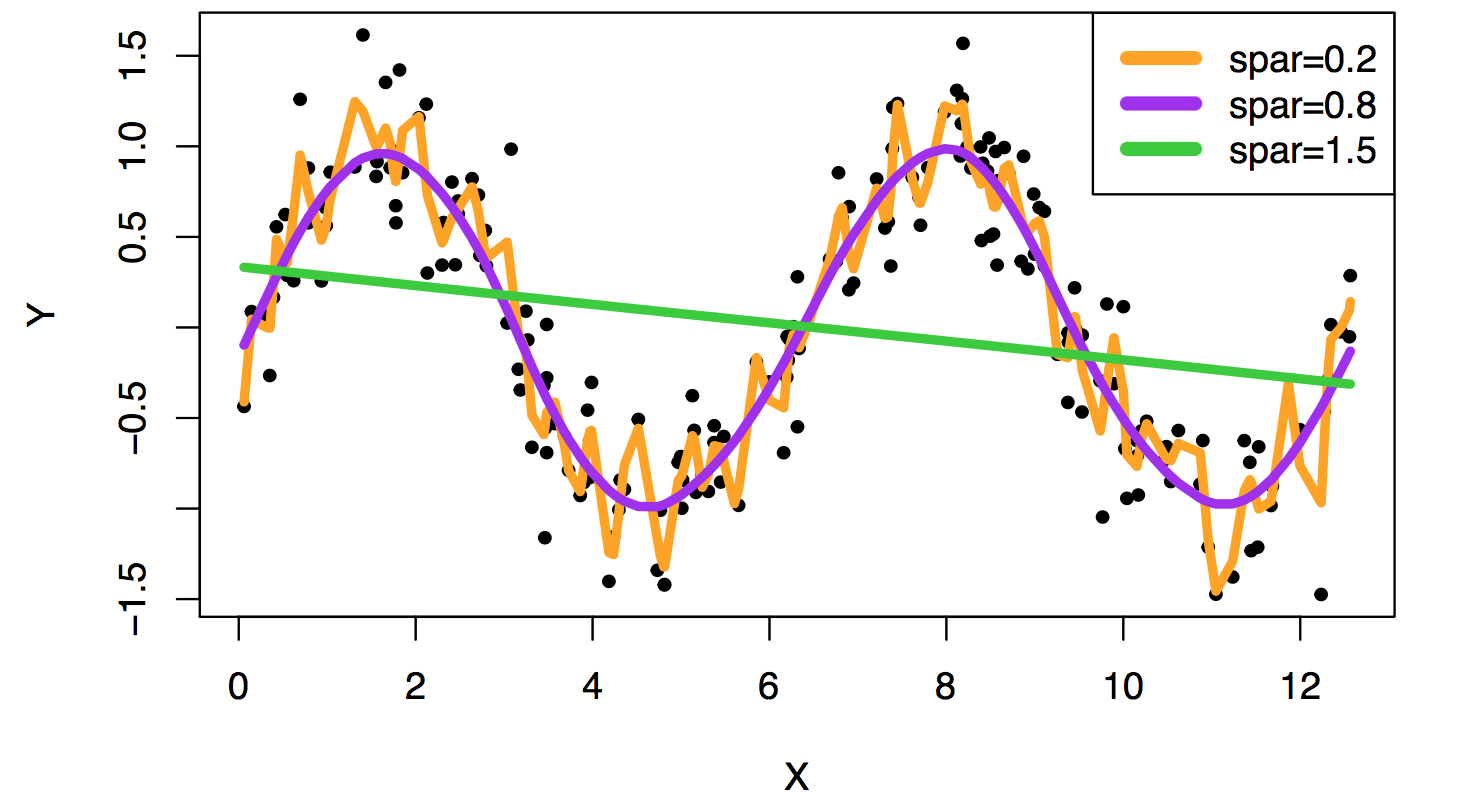
The overfitting means that you fit a too complex model to the data so that although the fitted curve is close to most of the observations, the actual prediction is very bad. For instance, the following picture shows the fitted result using a smoothing/cubic spline (here the quantity spar is related to $\lambda$):

This data is generated from a sine function plus a small noise. When $\lambda$ is too small (orange curve), we fit a very complicated model to the data, which does not capture the right structure. On the other hand, when $\lambda$ is too large (green curve), we fit a too simple model (a straight line), which is also bad in predicting the actual outcome. When $\lambda$ is too small, it is called overfitting (orange curve) whereas when $\lambda$ is too large, it is called underfitting (green curve). In fact, overfitting is similar to undersmoothing and underfitting is similar to oversmoothing. In regression analysis, people prefer to use overfitting and underfitting to describe the outcome and in density estimation, people prefer to use undersmoothing and oversmoothing.

Finding a regression estimator using a criterion with a fitting to the data plus a penalty on the complexity is called a penalized regression. In the case of regression tree, let \[\mathcal{M}_{\sf Tree} = \{\mbox{all possible regression trees}\}\] be the collection of all possible regression trees. We can rewrite equation $\eqref{eq::regTree}$ as \[\widehat{m}_{\sf Tree} =\underset{m\in\mathcal{M}_{\sf Tree}}{{\sf argmin}} \,\,\frac{1}{n}\sum_{i=1}^n(Y_i - m(X_i))^2 + \mathcal{P}_\lambda(m),\] where $\mathcal{P}_\lambda(m) = \lambda \times \mbox{number of regions in $m$}$. Thus, with the penalty on the number of regions, the regression tree is a penalized regression approach.

For any penalized regression approach, there is an abstract expression for them: \[\begin{equation} \widehat{m} = \underset{m\in\mathcal{M}}{{\sf argmin}} \,\,\frac{1}{n}\sum_{i=1}^n(Y_i - m(X_i))^2 + \mathcal{P}_\lambda(m), \label{eq::penalty} \end{equation}\] where $\mathcal{M}$ is a collection of regression estimators and $\mathcal{P}_\lambda(m)$ is the amount of penalty imposed for a regression estimator $m\in\mathcal{M}$ and $\lambda$ is a tuning parameter that determines the amount of penalty. The penalized regression always has a fitting part (e.g., $\frac{1}{n}\sum_{i=1}^n(Y_i - m(X_i))^2$) and a penalized part (also called regularized part) $\mathcal{P}_\lambda(m)$. The fitting part makes sure the model fits the data well while the penalized part guarantees that the model is not too complex. Thus, the penalized regression often leads to a simple model with a good fitting to the data.

Spline

Smoothing spline is a famous example in penalized regression methods. Here we consider the case of univariate regression (i.e., the covariate $X$ is univariate or equivalently, $d=1$) and focus on the region where the covariates belongs to $[0,1]$. Namely, our data is $(X_1,Y_1),\cdots, (X_n,Y_n)$ with $X_i\in [0,1]\subset \mathbb{R}$ for each $i$.

Let $\mathcal{M}_2$ denote the collection of all univariate functions with second derivative on $[0,1]$. The cubic (smoothing) spline finds an estimator \[\begin{equation} \widehat{m} = \underset{m\in\mathcal{M}_2}{{\sf argmin}} \,\,\frac{1}{n}\sum_{i=1}^n(Y_i - m(X_i))^2 +\lambda\int_{0}^1|m''(x)|^2 dx. \label{eq::sp} \end{equation}\] In the cubic spline the penalty function is $\lambda\int_{0}^1|m''(x)|^2 dx$, which imposes restriction on the smoothness – the curve $m(x)$ cannot change too drastically otherwise the second derivatives will be large. Thus, the cubic spline leads to a smooth curve but fits to the data well.

Why is the estimator $\widehat{m}$ called a cubic spline? This is because it turns out that $\widehat{m}$ is a piecewise polynomial function (spline) with degree of $3$. Namely, there exists knots $\tau_1<\cdots<\tau_K$ such that for $x\in (\tau_k, \tau_{k+1})$, \[\widehat{m}(x) = \gamma_{0,k}+\gamma_{1,k}x + \gamma_{2,k}x^2 +\gamma_{3,k}x^3,\] for some $\gamma_{0,k},\cdots, \gamma_{3,k}$ with restriction that $\widehat{m}(x)$ has continuous second derivatives at each knot. In the case of cubic spline, it turns out that the knots are just data points.

The representation of a cubic spline is often done using some basis function. Here we will introduce a simple basis called the truncated power basis. Let $X_{(1)}<X_{(2)}<\cdots<X_{(n)}$ be the ordered statistics of $X_1,\cdots, X_n$. In the cubic spline, the knots are \[\tau_1 = X_{(1)},\tau_2 = X_{(2)},\cdots, \tau_n = X_{(n)}.\]

The truncated power basis uses a collection of functions \[h_1(x) = 1, h_2(x) = x, h_3(x) = x^2, h_4(x) = x^3,\] and \[h_{j}(x) = (x-\tau_{j-4})^3_+,\quad j=5,6,\cdots, n+4,\] where $(x)_+ = \max\{x,0\}$. Then the estimator $\widehat{m}$ can be written as \[\widehat{m}(x) = \sum_{j=1}^{n+4} \widehat\beta_j h_j(x),\] for some properly chosen $\widehat\beta_j$.

How do we compute $\widehat\beta_1,\cdots, \widehat\beta_{n+4}$? They should be chosen using equation $\eqref{eq::sp}$. Here is how we will compute it. Define an $n\times (n+4)$ matrix $\mathbb{H}$ such that \[\mathbb{H}_{ij} = h_j(X_i)\] and an $(n+4)\times (n+4)$ matrix $\Omega$ with \[\Omega_{ij} = \int_0^1 h''_i(x)h''_j(x)dx.\] In this case, we define $m(x) = \sum_{j=1}^{n+4} \beta_j h_j(x)$ so the criterion in the right-hand side of $\eqref{eq::sp}$ becomes \[\begin{align*} \frac{1}{n}\sum_{i=1}^n(Y_i - m(X_i))^2 &+\lambda\int_{0}^1|m''(x)|^2 dx\\ &= \frac{1}{n}\sum_{i=1}^n\left(Y_i - \sum_{j=1}^{n+4}\beta_jh_j(X_i)\right)^2 +\lambda\int_{0}^1\left(\sum_{j=1}^{n+4} \beta_j h_j(x)\right)\left(\sum_{\ell=1}^{n+4} \beta_\ell h_\ell(x)\right) dx\\ &= \|\mathbb{Y} - \mathbb{H}\beta\|^2 + \lambda\beta^T \Omega \beta\\ & = R_n(\beta) \end{align*}\] where $\mathbb{Y} = (Y_1,\cdots, Y_n)$ and $\beta = (\beta_1,\cdots, \beta_{n+4})$. Thus, \[\widehat{\beta} = {\sf argmin}_\beta R_n(\beta) = ( \mathbb{H}^T \mathbb{H} + \lambda\Omega)^{-1} \mathbb{H}^T\mathbb{Y}.\]

Given a point $x$, let $H(x) = (h_1(x), h_2(x),\cdots, h_{n+4}(x))$ be an $(n+4)$-dimensional vector. Then the predicted value $\widehat{m}(x)$ has a simple form: \[\widehat{m}(x) = H^T(x) \widehat{\beta} = H^T(x)( \mathbb{H}^T \mathbb{H} + \lambda\Omega)^{-1} \mathbb{H}^T\mathbb{Y} = \sum_{i=1}^n \ell_i(x)Y_i,\] where \[\ell_i(x) = H^T(x)( \mathbb{H}^T \mathbb{H} + \lambda \Omega)^{-1} \mathbb{H}^Te_i,\] with $e_i = (0,0,\cdots, 0,\underbrace{1}_\text{$i$-th coordinate},0,\cdots, 0)$ is the unit vector in the $i$-th coordinate. Therefore, again the cubic spline is a linear smoother.

Note that when the sample size $n$ is large, the spline estimator behaves like a kernel regression in the sense that \[\ell_i(x) \approx \frac{1}{p(X_i)h(X_i)}K\left(\frac{X_i-x}{h(X_i)}\right)\] and \[h(x) = \left(\frac{\lambda}{np(x)}\right)^{1/4},\quad K(x) = \frac{1}{2} \exp\left(-\frac{|x|}{\sqrt{2}}\right)\sin\left(\frac{|x|}{\sqrt{2}}+\frac{\pi}{4}\right).\] This is formally stated in the following paper: