A contingency table is a powerful tool in data analysis for comparing two categorical variables. Although it is designed for analyzing categorical variables, this approach can also be applied to other discrete variables and even continuous variables. We start with a simple example.
Example 1.1 Suppose we have two categorical variables: gender (male or female) and handedness (right or left handed). Assume that we conduct a simple random sampling and obtain a size \(100\) data. We can then summarize our data using the following \(2\times 2\) table:
| Right-handed | Left-handed | |
|---|---|---|
| Male | \(43\) | \(9\) |
| Female | \(44\) | \(4\) |
Such a table is called a \(2\times 2\) contingency table.
Sometimes you may see people augment the table with the total sums:
| Right-handed | Left-handed | Total | |
|---|---|---|---|
| Male | \(43\) | \(9\) | \(52\) |
| Female | \(44\) | \(4\) | \(48\) |
| 1-4 Total | \(87\) | \(13\) | \(100\) |
The contingency table elegantly summarizes the information about our data and may be one of the most common data analysis tools.
A general \(2\times 2\) contingency table will be as follows:
| \(Y=y_1\) | \(Y=y_2\) | |
|---|---|---|
| \(X=x_1\) | \(a\) | \(b\) |
| \(X=x_2\) | \(c\) | \(d\) |
Here the two variables are \(X\) and \(Y\) and each of them has two possible categories.
When the two variables have more than two categories, they can still be presented in a contingency table but the table will be larger. For instance, if \(X\) has \(n\) distinct categories and \(Y\) has \(m\) categories, the contingency table will be a \(n\times m\) table as follows:
| \(Y=y_1\) | \(Y=y_2\) | \(\cdots\) | \(Y=y_m\) | Total | |
|---|---|---|---|---|---|
| \(X=x_1\) | \(T_{11}\) | \(T_{12}\) | \(\cdots\) | \(T_{1m}\) | \(R_1\) |
| \(X=x_2\) | \(T_{21}\) | \(T_{22}\) | \(\cdots\) | \(T_{2m}\) | \(R_2\) |
| \(\cdots\) | \(\cdots\) | \(\cdots\) | \(\cdots\) | \(\cdots\) | \(\cdots\) |
| \(X=x_n\) | \(T_{n1}\) | \(T_{n2}\) | \(\cdots\) | \(T_{nm}\) | \(R_n\) |
| Total | \(C_1\) | \(C_2\) | \(\cdots\) | \(C_m\) | \(N\) |
The quantity \(T_{ij}\) is the number of observations with \(X=x_i\) and \(Y=y_j\) and \(R_i = \sum_{j=1}^n T_{ij}\) is the sum of the \(i\)-th row and \(C_j = \sum_{i=1}^n T_{ij}\) is the sum of the \(j\)-th column and \(N = \sum_{i,j} T_{ij}\) is the sample size.
Example 2. Here is an example of a \(2\times 4\) contingency table2:
| Outcome | |||||
| Diet | Cancers | Fatal Heart Disease | Non-Fatal Heart Disease | Healthy | Total |
| AHA | 15 | 24 | 25 | 239 | 303 |
| Mediterranean | 7 | 14 | 8 | 273 | 302 |
| Total | 22 | 38 | 33 | 512 | 605 |
As we have mentioned, the contingency table is a tool for analyzing two variables. Given two variables, a common question we often ask is: are these two variables dependent? The contingency table provides us a simple way to test such a hypothesis. Here is a key insight. If the null hypothesis is correct, the two variables will be independent. Thus, the ratio \(\frac{T_{ij}}{N}\) should be close to \(\frac{R_i}{N}\times \frac{C_j}{N}\) which implies \(T_{ij}\) should be comparable to \(\frac{R_iC_j}{N}\). We will call \(T_{ij}\) the observed frequencies and \(\frac{R_i C_j}{N}= E_{ij}\) the expected (theoretical) frequencies.
The Pearson’s \(\chi^2\) test utilizes this fact and uses the test statistic \[\chi^2 = \sum_{i,j} \frac{(T_{ij}-E_{ij})^2}{E_{ij}}.\] And it can be shown that this test statistic has an asymptotic distribution of a \(\chi^2\) distribution with degrees of freedom \((n-1)(m-1)\). Thus, the p-value is \[{\sf pvalue} = 1-\Phi_{\chi^2_{(n-1)(m-1)}}(\chi^2),\] where \(\Phi_{\chi^2_{\nu}}(x)\) is the CDF of a \(\chi^2\) distribution with \(\nu\) degrees of freedom. The reason why \(\chi^2\) approximates a \(\chi^2\) distribution with degrees of freedom \((n-1)(m-1)\) is due to the likelihood ratio test and multinomial distribution.
Example 2 (revisited). Now we test if the diet and the outcome are independent in the data of Example 2. By calculating the expected frequencies, we obtain a new table where the number in the parentheses denotes the expected frequencies:
| Outcome | |||||
| Diet | Cancers | Fatal Heart Disease | Non-Fatal Heart Disease | Healthy | Total |
| AHA | 15 (11.02) | 24 (19.03) | 25 (16.53) | 239 (256.42) | 303 |
| Mediterranean | 7 (10.98) | 14 (18.97) | 8 (16.47) | 273 (255.58) | 302 |
| Total | 22 | 38 | 33 | 512 | 605 |
This leads to the Pearson’s \(\chi^2\) test statistic \(\chi^2 = 16.55\) and comparing this to a chi-square distribution with \((2-1)(4-1) = 3\) degree of freedom, we obtain a p-value \(0.0009\).
Example 1 (revisited). We check whether gender and handedness in Example 1 are independent or not. Here is the table with expected frequencies:
| Right-handed | Left-handed | Total | |
|---|---|---|---|
| Male | \(43 (45.24)\) | \(9 (6.76)\) | \(52\) |
| Female | \(44 (41.76)\) | \(4 (6.24)\) | \(48\) |
| 1-4 Total | \(87\) | \(13\) | \(100\) |
This yields a test statistic \(\chi^2 = 1.78\) and by comparing to a \(\chi^2\) distribution with degree of freedom \(1\), we obtain a p-value \(0.1821\).
Remark. (On degrees of freedom) Why in testing the independence of an \(n\times m\) contingency table is the degrees of freedom of the \(\chi^2\) distribution \((n-1)(m-1)\)? Why is it called degrees of freedom? Here is a simple explanation. At first, the contingency table has a total of \(nm\) variables. All these variables can change freely without any restriction so the initial degrees of freedom is \(nm\). When we test independence, this hypothesis imposes some restriction on the variables so not all variables can change freely if the null hypothesis \(H_0\) is correct. In the model of the null hypothesis, the \(nm\) variables (cells in the table) can be expressed by the products of \(R_i\) and \(C_j\) for \(i=1,\cdots, n\) and \(j=1,\cdots, m\). Thus, this model (the model under \(H_0\)) has \(n+m\) variables. However, not all these \(n+m\) variables are free – the sum of \(R_i\)’s and the sum of \(C_j\)’s will be the same. So these \(n+m\) variables only contain \(n+m-1\) free variables. Namely, the degrees of freedom of \(R_1,\cdots,R_n, C_1,\cdots, C_m\) is \(n+m-1\). Because the model under \(H_0\) has a degree of freedom \(n+m-1\) and the model without any restriction has a degree of freedom \(nm\), the remaining degrees of freedom is \(nm - (n+m-1) = nm-n-m+1 = (n-1)(m-1)\).
Remark. In addition to the Pearson’s \(\chi^2\) test, there is another approach called Fisher’s exact test. We do not have time to cover it here but I would highly recommend reading the following article on Wikipedia: https://en.wikipedia.org/wiki/Fisher%27s_exact_test.
A common parametric model for modeling the contingency table is the log-linear model. Because in the contingency table, each cell \(T_{ij}\) is a nonnegative integer. Thus, a natural model for \(T_{ij}\) is a Poisson distribution. Namely, we assume that \(T_{ij}\sim {\sf Poisson} (\lambda_{ij})\) for some rate parameter \(\lambda_{ij}\) for \(i=1,\cdots, n\) and \(j=1,\cdots,m\).
The log-linear model uses a better parametrization of \(\lambda_{ij}\) by rewriting it as \[\begin{equation} \log (\lambda_{ij}) = \mu+\alpha_i +\beta_j +\gamma_{ij} \label{eq::loglinear} \end{equation}\] with the following constraints: \[0 = \sum_{i=1}^n \alpha_i =\sum_{j=1}^m \beta_j = \sum_{i=1}^n\gamma_{ij}= \sum_{j=1}^m\gamma_{ij}.\] These constraints are applied to ensure there is no overparametrization (more variables than we need).
What are the benefits of using the parametrization in equation \(\eqref{eq::loglinear}\)? The parameters in equation \(\eqref{eq::loglinear}\) have simple interpretations: \(\mu\) stands for the overall effect, \(\alpha_i\) is the effect from variable \(X\) being in the \(i\)-th category, \(\beta_j\) is the effect from variable \(Y\) being in the \(j\)-th category, and \(\gamma_{ij}\) is the remaining individual effect.
The log-linear model also has a good way of expressing independence. The two variables are independent if \[\gamma_{ij} = 0 \,\,\forall\,\, i=1,\cdots, n, j=1,\cdots, m.\] Namely, we can rewrite the independence as setting certain parameters to \(0\). The estimation of these parameters is often done using a maximum likelihood procedure3, which is beyond the scope of this course.
The log-linear model can be easily extended to three variables or even more variables. When we are comparing more than two variables, contingency table may not be easily displayed. However, the log-linear model still has an elegant form. In the case of three variables, we have a table \(T_{ijk}\) where \(i=1,\cdots,n\), \(j=1,\cdots, m\), and \(k=1,\cdots, p\) (first variable has \(n\) categories; second variable has \(m\) categories; third variable has \(p\) categories). The log-linear model will be \[\begin{align*} T_{ijk} &\sim {\sf Poisson}(\lambda_{ijk})\\ \log (\lambda_{ijk}) &= \mu+\alpha_i +\beta_j +\gamma_{k} + \delta_{ij} + \rho_{ik} + \kappa_{jk} + \xi_{ijk} \end{align*}\] with constraints to avoid overparametrization.
If you are interested in learning more about log-linear model and contingency table, I would recommend the following online source: https://onlinecourses.science.psu.edu/stat504/node/117.
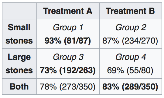
Simpson’s paradox is perhaps one of the most famous paradoxes in statistics. Here is a simple example illustrating it. Consider the following \(2\times 2\) contingency table:
This is a famous dataset about kidney stone treatments from Wikipedia4 This table is not the conventional contingency table we are seeing. It is a table describing the success rate of each case and the number in parentheses shows the number of observations in that scenario. For instance, Group 1 is the case where the individuals have small stones in their kidney and they received treatment A and there are \(87\) individuals in this scenario and the treatment works in \(81\) out of \(87\) individuals. The entire dataset consists of two treatments (A or B) and two types of kidney stones (small and large) and 700 individuals.
Now, if we ignore the types of stones and just compare the success rate of the two treatments (comparing the bottom row), treatment B has a higher success rate. However, if we take the type of stones into account, then regardless of the type of stones, treatment A is always better than treatment B! This paradoxical phenomenon is called the Simpson’s paradox.
Why does this happen? The main reason is that the two variables being considered here, the treatment and the type of stones, are highly dependent. As you can see, treatment A is often applied to large stone individuals whereas treatment B is often used to treat small stone patients. Such a dependence may cause Simpson’s paradox. Thus, when designing an experiment, we often need to check for dependence among our variables. This is why the methods we just learned in analyzing a contingency table are very useful.
In addition to the test of independence in a contingency table, the Pearson’s \(\chi^2\) test can be applied to the goodness-of-fit test as well5. It is a common approach for testing the distribution of a discrete random variable or a categorical random variable. We start with a simple example.
Example 3. A normal die (\(6\)-sided) is thrown \(60\) times and we record the number of each time. Here is the outcome of the \(60\) tosses:
| Number face up: | 1 | 2 | 3 | 4 | 5 | 6 |
|---|---|---|---|---|---|---|
| Counts: | 5 | 8 | 9 | 8 | 10 | 20 |
Is this die a fair die (i.e., all faces have equal probability facing up)?
To test such a hypothesis, again we use the Pearson’s \(\chi^2\) statistic. Here the expected frequency is \(10\) for every case. We modify the previous table by adding the expected frequencies in parentheses:
| Number face up: | 1 | 2 | 3 | 4 | 5 | 6 |
|---|---|---|---|---|---|---|
| Counts: | 5 (10) | 8 (10) | 9 (10) | 8 (10) | 10 (10) | 20 (10) |
The Pearson’s \(\chi^2\) statistic is \[\chi^2 = \sum_{i} \frac{(O_i-E_i)^2}{E_i} = \frac{(5-10)^2}{10}+\frac{(8-10)^2}{10}+ \frac{(9-10)^2}{10}+\frac{(8-10)^2}{10}+\frac{(10-10)^2}{10}+\frac{(20-10)^2}{10}=13.4,\] where \(O_i\) is the observed outcomes whereas \(E_i\) is the expected outcomes.
As for the reference distribution, it will follow a \(\chi^2\) distribution with degrees of freedom \(5\). The degrees of freedom \(5 = 6-1\), where \(6\) is the total number of free variables (the frequencies of each number being face up) and the minus \(1\) is from the degree of freedom in \(H_0:\) there is only one frequency in \(H_0\) (the average frequency). Thus, the p-value in this case is about \(0.02\).
Essentially, the Pearson’s \(\chi^2\) test for the goodness-of-fit test uses the same test statistic as for the independence test. The challenging part is to determine the number of degrees of freedom of the reference \(\chi^2\) distribution. Here is a simple rule for calculating the degrees of freedom: it is the total number of free parameters minus the number of free parameters in \(H_0\).
This example is from wikipedia: https://en.wikipedia.org/wiki/Contingency_table.↩︎
This data is from the Mediterranean Diet and Health case study http://onlinestatbook.com/2/chi_square/contingency.html.↩︎
https://en.wikipedia.org/wiki/Maximum_likelihood_estimation↩︎
https://en.wikipedia.org/wiki/Pearson%27s_chi-squared_test↩︎