Useful reference:

• Wasserman, L. (2018). Topological data analysis. Annual Review of Statistics and Its Application, 5, 501-532.

• Chapter 14.3 of Friedman, J., Hastie, T., & Tibshirani, R. (2001). The elements of statistical learning. New York: Springer series in statistics.

Introduction

Clustering is one of the most important tasks in data analysis. The objective of clustering is to separate data into groups such that observations within the same groups are similar.

Because there is no formal definition of a cluster, there are several different clustering approaches that attempt to define similarity using different notions.

We will start with density-based clustering methods that define clusters through a density function. In this case, a density estimator leads to a clustering method. Then we discuss clustering methods that directly apply to the observations without using a density estimator although many of them implicitly use the notion of density.

Mode clustering

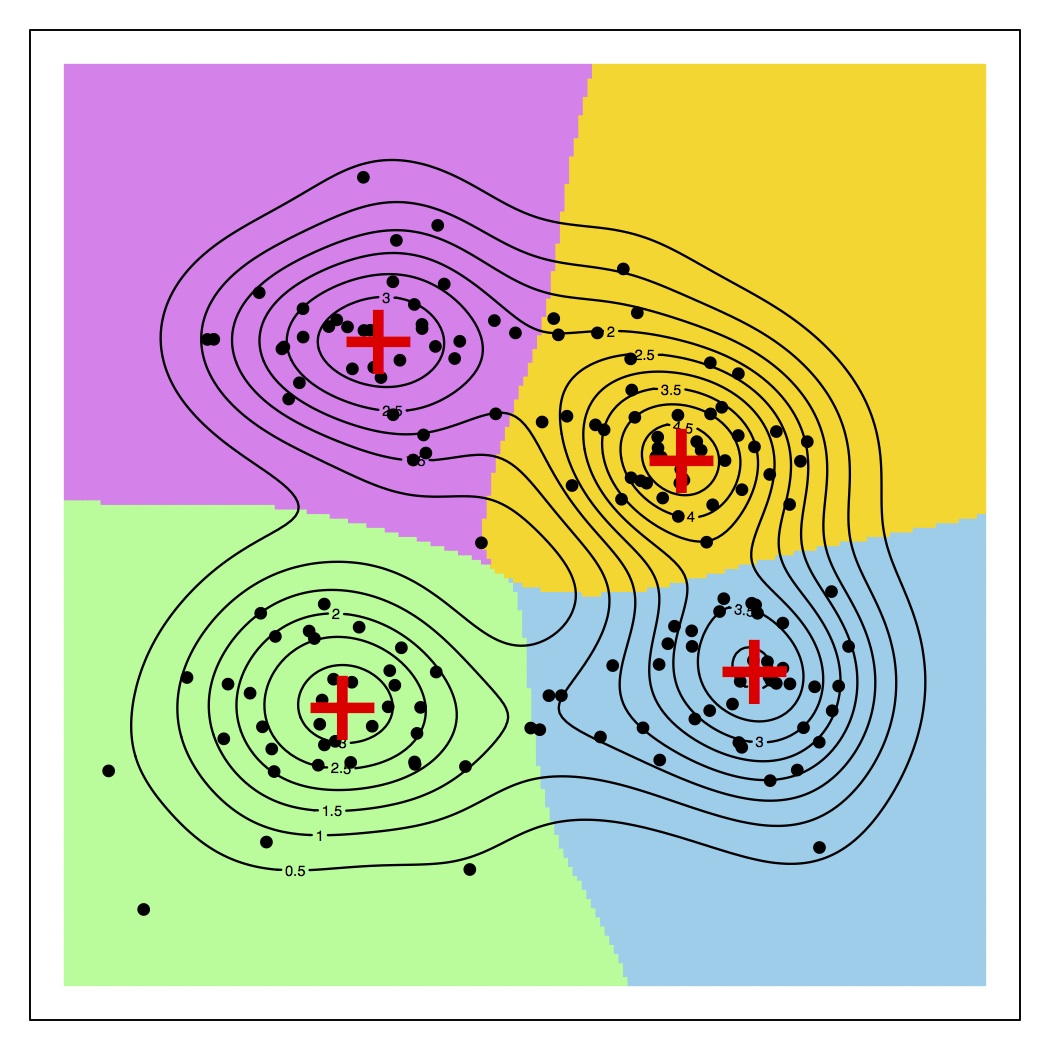
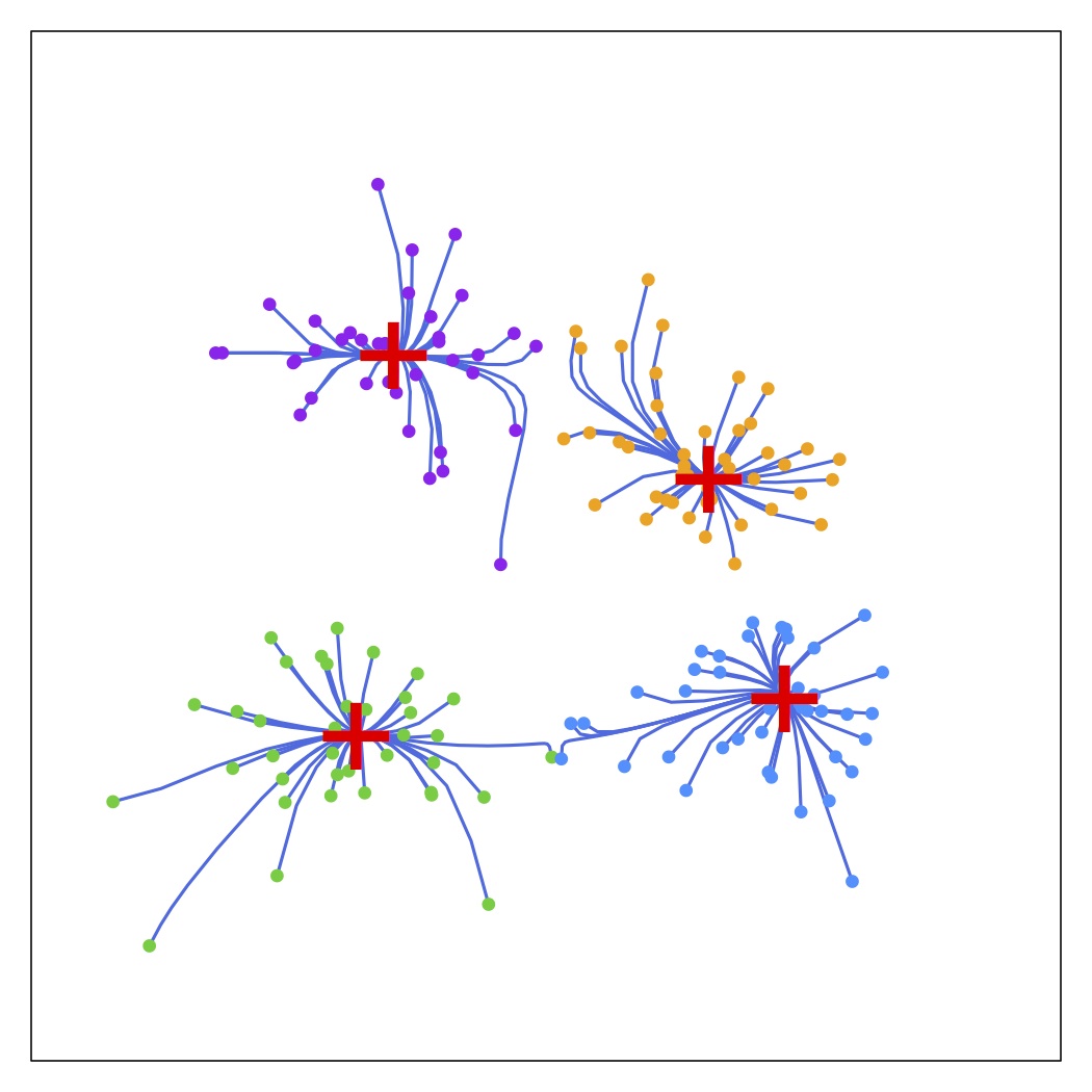
The mode clustering forms clusters by using the gradient flow of a PDF. Consider a PDF \(p(x)\) that is smooth. Starting at point \(x\), we define a gradient ascent flow \(\pi_x:\mathbb{R}\mapsto \mathbb{R}^d\) such that \[\pi_x(0) = x,\quad \pi'_x(t) = \nabla p(\pi_x(t)).\] You can easily verify that the flow \(\pi_x\) is the density gradient ascent flow starting at point \(x\).

When \(p(x)\) is a Morse function (all critical points are non-degenerated, i.e., Hessian matrix at each critical point has non-zero eigenvalues), the destination \[\pi_x(\infty) = \lim_{t\rightarrow\infty}\pi_x(t)\] belongs to one of the local modes of \(p(x)\) except for a set of Lebesgue measure \(0\). We then use the destination of the gradient flow \(\pi_x(\infty)\) to cluster the entire sample space. Namely, points whose gradient flow converges to the same destination belong to the same cluster. Let \(M\) be the collection of all local modes of \(p\) and for any point \(m\in M\), we define \[D(m) = \{x: \pi_x(\infty)=m\}\] be the basin of attraction of \(m\). The collection \(\{D(m): m\in M\}\) can be viewed as a population clustering of the entire sample space. When a set of observations \(X_1,\cdots, X_n\) are given, we can use the basin that each observation falls into to cluster observations.

In practice, we do not know the population PDF. Instead, we have a random sample \(X_1,\cdots, X_n\sim p\). So we will estimate the PDF first and then use the gradient flow of the density estimator to perform mode clustering. In particular, we often use the kernel density estimator (KDE) \[\widehat p_h(x) = \frac{1}{nh^d}\sum_{i=1}^n K\left(\frac{X_i-x}{h}\right)\] and its derivative to perform mode clustering.

When we use the Gaussian kernel, the gradient descent can be done by using the mean-shift algorithm. Suppose \(x^{(0)}\) is the initial point that we want to start the gradient flow with. We updates it by \[\begin{equation} x^{(t+1)} = \frac{\sum_{i=1}^nX_i K\left(\frac{X_i-x^{(t)}}{h}\right)}{\sum_{j=1}^n K\left(\frac{X_j-x^{(t)}}{h}\right)}. \end{equation}\] You can show that this iteration is indeed a gradient ascent algorithm and the convergent point \(x^{(\infty)}\) will be a local mode of \(\widehat p_h\) for most initial points. When the mode clustering is done by the mean shift algorithm, it is also called mean-shift clustering.

Using the mean-shift algorithm, we can define the sample basin of attraction \[\widehat D(m) = \{x: \widehat\pi_x(\infty)=m\},\] where \(\widehat\pi_x(t)\) is the gradient flow of \(\widehat p_h\) and \(m \in \widehat M_h\) such that \(\widehat M_h\) is the local modes of \(\widehat p_h\). We set \(X_i\) into a cluster \(m\) if \(X_i\in \widehat D(m)\).

Here is a paper that you may want to read if you are interested in the idea of mode clustering:

Chacón, J. E. (2015). A population background for nonparametric density-based clustering. Statistical Science, 30(4), 518-532.

Stability of mode clustering

Since the mode clustering can be applied to a population PDF and what we computed is the sample version of the mode clustering, we can define the concept of convergence of clustering in this case– we want the sample clusters to converge to the population clusters.

There are two ways to quantify the convergence of a mode clustering result. The first one is to show that the convergent points (i.e., local modes) in \(\widehat p_h\) converge to the local modes in \(p\). The second one is to show that the two partitions of the observations agree with each other (often measured by the Rand index¹).

To quantify the convergence of local modes, we use the Hausdorff distance. For two sets \(A\) and \(B\), their Hausdorff distance is \[{\sf Haus}(A,B) = \max\left\{\sup_{x\in A}d(x,B), \sup_{x\in B}d(x,A)\right\}.\] You can view the Hausdorff distance as an \(L_\infty\) distance of sets.

The above theorem is from the following paper:

Chen, Y. C., Genovese, C. R., & Wasserman, L. (2016). A comprehensive approach to mode clustering. Electronic Journal of Statistics, 10(1), 210-241.

Note that the smoothing bandwidth requirement is stronger than the convergence rate. The requirement \(h\rightarrow 0,\frac{\log n}{nh^{d+4}}\rightarrow 0\) is to make sure that the Hessian matrix is consistently estimated so that the modes can be consistently estimated. Here is an intuitive explanation on why we need a consistent estimate of the second derivative but the rate only depends on the first derivative. Let \(m\) be a local mode of \(p\) and \(\widehat m_h\) be a local mode of \(\widehat p_h\) that is closest to \(m\). By definition of local modes, we have \[\nabla p(m) = 0 = \nabla \widehat p_h(\widehat m_h).\] Thus, by the Taylor expansion, \[\begin{align*} \nabla \widehat p_h(m) - \underbrace{\nabla p(m)}_{=0} & =\nabla \widehat p_h(m) - \nabla \widehat p_h(\widehat m_h)\\ & = \nabla \nabla \widehat p_h(m) (m - \widehat m_h) + O(\|\widehat m_h-m\|^2). \end{align*}\] Ignoring the second order term, we obtain \[\widehat m_h - m = [ \nabla \nabla \widehat p_h(m)]^{-1} (\nabla \widehat p_h(m) - \nabla p(m)).\] When the second derivatives converge, the first term converges to \([ \nabla \nabla p(m)]^{-1}\), which will be of a constant order. So the rate is determined by \(\nabla \widehat p_h(m) - \nabla p(m)\), the gradient estimation rate. This analysis also reveals the importance of being a Morse function–we need the Hessian matrix to be invertible around local modes, i.e., eigenvalues of the Hessian matrix are all non-zero.

Thus, when the density function is smooth, the estimated local modes converge to the population local modes.

Let \(\mathbb{C}(X_i)\) be the cluster label of \(X_i\) using the population mode clustering and \(\widehat{\mathbb{C}}(X_i)\) be the cluster label of \(X_i\) using the sample mode clustering. Then the Rand index between the population and sample mode clustering is \[\begin{align*} {\sf rand}(\mathbb{C},\widehat{\mathbb{C}}) &= \frac{1}{{n\choose 2}} \sum_{i,j=1}^n I(\mathbb{C}(X_i) = \mathbb{C}(X_j), \widehat{\mathbb{C}}(X_i) \neq \widehat{\mathbb{C}}(X_j))+ I(\mathbb{C}(X_i) \neq \mathbb{C}(X_j), \widehat{\mathbb{C}}(X_i) = \widehat{\mathbb{C}}(X_j))\\ & = \mbox{ratio of pairs on which the two clustering methods disagree.} \end{align*}\]

The above theorem is from the following paper:

Chen, Y. C., Genovese, C. R., & Wasserman, L. (2017). Statistical inference using the morse-smale complex. Electronic Journal of Statistics, 11(1), 1390-1433.

Namely, asymptotically the sample mode clustering and population mode clustering return the same partition of the data (except only a small fraction of observations).

Level set clustering

Another density-based clustering method is the level set clustering. The idea is very simple. Consider the \(\lambda\)-upper level set: \[L_\lambda =\{x: p(x)\geq \lambda\}.\] Namely, \(L_\lambda\) is the collection of regions where the PDF is greater than or equal to \(\lambda\).

When \(p\) has multiple local modes, some level sets would lead to several connected components. The level set clustering groups observations into the same cluster if they are all on the same connected component.

Again, in practice we estimate the PDF by a density estimator and use the estimated level set to perform clustering. Namely, suppose that \(\widehat p\) is a density estimator. Then we use \[\widehat L_\lambda = \{x: \widehat p(x)\geq \lambda\}\] as an estimator of \(L_\lambda\) and the corresponding connected components to cluster observations.

Sometimes estimating the level set itself is of research interest since level sets are regions characterizing high density areas. In addition to clustering, the idea of level sets can also be applied to perform anomaly detection – observations falling in the low density area \(L_\lambda^C = \{x: p(x)<\lambda\}\) will be classified as anomalies.

I would recommend the following two papers for learning more about level set clustering:

Rinaldo, A., Singh, A., Nugent, R., & Wasserman, L. (2012). Stability of density-based clustering. Journal of Machine Learning Research, 13(Apr), 905-948.
Rinaldo, A., & Wasserman, L. (2010). Generalized density clustering. The Annals of Statistics, 38(5), 2678-2722.

Stability of level sets

There are many theoretical results on the stability of a level set. Often a key assumption we need to make is the behavior of \(p(x)\) around \(L_\lambda\). As you may expect, if \(p(x)\) is close to flat around \(L_\lambda\), the level set is unstable whereas if \(p(x)\) has a high gradient around \(L_\lambda\), the level set is stable.

Let \(\epsilon = \|p_n - p\|_{\infty}\). Consider a point \(x\in p_n\). It is easy to see that \(p_n(x) = \lambda\) and \(p(x)\in [ \lambda - \epsilon, \lambda+\epsilon]\).

Moreover, because of assumption (G) and the fact that \(p\) has bounded second derivative, for any point \(x\) with \(p(x) \in [ \lambda - \epsilon, \lambda+\epsilon]\), the gradient \(\|\nabla p(x)\|\geq \frac{1}{2}g_0\) (think about why this is the case). Note that \(\frac{1}{2}\) can be replaced by any number that is strictly less than \(\frac{1}{2}\).

Now we define a gradient ascent flow \(\pi_x(t)\) \[\pi_x(0) = x,\quad \pi'_x(t) = \nabla p(\pi_x(t)).\] Since \(\pi_x(t)\) is a gradient ascent flow, the density value \(p(\pi_x(t))\) satisfies \[\frac{d}{dt} p(\pi_x(t)) = [\nabla p(\pi_x(t))]^T \pi_x'(t) = \|\nabla p(\pi_x(t))\|^2 \geq \frac{1}{4}g^2_0>0\] whenever \(p(\pi_x(t)) \in [ \lambda - \epsilon, \lambda+\epsilon]\).

Since the density is increasing, let \(\tau\) be the time such that \(p(\pi_x(\tau)) = \lambda\). Then \[\begin{align*} \lambda - p(x) & = p(\pi_x(\tau)) - p(\pi_x(0))\\ & = \int_{t=0}^{t=\tau} \frac{d}{dt} p(\pi_x(t)) dt\\ &\geq \frac{1}{4}g^2_0 \tau. \end{align*}\] Because \(p_n(x) = \lambda\) and \(\epsilon = \|p_n - p\|_{\infty}\), the above inequality implies \[\epsilon\geq \frac{1}{2}g_0\tau\Rightarrow \tau \leq \frac{4\epsilon}{g^2_0}.\]

Thus, we obtain an upper on the time \(\tau\). Because \(\pi_x(\tau)\in L_\lambda\), \[\begin{align*} d(x, L_\lambda)&\leq\|\pi_x(\tau) - x\|\\ & = \|\pi_x(\tau) -\pi_x(0)\|\\ &\leq \int_{t=0}^{t=\tau} \|\pi_x'(t)\| dt\\ &\leq \tau \cdot g_{\max}, \end{align*}\] where \(g_{\max} = \sup_{x} \|\nabla p(x)\|\). So the upper bound on \(\tau\) implies \[d(x, L_\lambda) \leq \tau \cdot g_{\max}\leq \frac{4g_{\max}}{g_0^2} \epsilon.\] This works for every \(x\in L_{\lambda, n}\) so we have proved the result for the case of \(x\in L_{\lambda, n}\).

The same argument also applies to the case for \(x\in L_\lambda\) by exchanging \(L_\lambda\) and \(L_{\lambda, n}\). Thus, we have proved the result for both quantities in the Hausdorff distance so the proof is completed.

Note that there are a couple of alternative approach to derive the same bound as the above theorem under a similar condition. See the following papers for some examples

Cadre, B. (2006). Kernel estimation of density level sets. Journal of multivariate analysis, 97(4), 999-1023.
Cuevas, A., González-Manteiga, W., & Rodríguez-Casal, A. (2006). Plug-in estimation of general level sets. Australian & New Zealand Journal of Statistics, 48(1), 7-19.

It is possible to construct a confidence set of the level sets. One possible way is to use the following insight. Let \(t_\alpha\) be the \(1-\alpha\) quantile of \({\sf Haus}(\widehat L_\lambda, L_\lambda)\). Then \[P(L_\lambda \subset \widehat L_\lambda \oplus t_\alpha) \geq 1-\alpha\] so the set \(\widehat L_\lambda \oplus t_\alpha\) is a \(1-\alpha\) confidence set of \(L_\lambda\). The following paper derives the asymptotic theory and propose a bootstrap approach to construct a confidence set of \(L_\lambda\):

Chen, Y. C., Genovese, C. R., & Wasserman, L. (2017). Density level sets: Asymptotics, inference, and visualization. Journal of the American Statistical Association, 112(520), 1684-1696.

Level set by a probability mass

Instead of fixing a level \(\lambda\), sometimes we would like to construct a level set such that \(P(L_\lambda)\) covers \(1-\gamma\) probability. Namely, we specify \(1-\gamma\) first and then tune \(\lambda\) such that \(P(L_\lambda)\) covers a probability of \(1-\gamma\).

However, sometimes we cannot find an exact level \(\lambda\) such that the level set covers exactly \(1-\gamma\) probability. In this case, we will find the largest level \(\lambda\) such that we have at least \(1-\gamma\) probability. Namely, the level is defined as \[\lambda(\gamma) = \inf\{\lambda>0: P(L_\lambda)\geq 1-\gamma\}.\]

The probability level set can be defined using the level set of density ranking, a transform quantity from the PDF. Let \[\alpha(x) = P(x\geq X),\quad X\sim p\] be the probability that a new observation \(X\) has lower or equal density compared to the given point \(x\). With this, the level set \[\Gamma_\gamma = \{x: \alpha(x)\geq 1-\gamma\}\] has the property that \(P(\Gamma_\gamma) = 1-\gamma\) and \(\Gamma_\gamma = L_{\lambda(\gamma)}\).

We can estimate \(\alpha(x)\) by \[\widehat\alpha(x) = \frac{1}{n}\sum_{i=1}^n I(\widehat p(x)\geq \widehat p(X_i)).\] Under good conditions, \(\widehat\alpha(x)\) will be a consistent estimator of \(\alpha(x)\). In particular, the following theorem shows the convergence.

The smoothing bandwidth requirement is of the rate of estimating the Hessian matrix. We need the Hessian matrix to be consistently estimated because of the stability of local modes.

Note that the density ranking can be applied to singular distribution (the PDF does not even exist). You can find more details from

Chen, Y. C. (2019). Generalized cluster trees and singular measures. The Annals of Statistics, 47(4), 2174-2203.

The level set indexed by the probability mass has another formulation. It can be interpreted as the minimum volume set. You can show that \(\Gamma_\gamma\) is a feasible solution of the following minimization problem \[\text{ minimize}\quad {\sf Vol}(A),\quad \mbox{subject to } P(A) \geq 1-\gamma.\] When the PDF exists and is smooth, any solution to the above minimization problem is the same as \(\Gamma_\gamma\) except for a set of \(0\) Lebesgue measure (volume).

Because the level set \(\Gamma_\gamma\) has the above minimum volume property, it is often used as a prediction region–given an accuracy of \(1-\gamma\), \(\Gamma_\gamma\) is the best prediction region we can have in the sense that the size is minimal.

Cluster trees

In level set clustering, a common problem is how to choose the level \(\lambda\) (or the probability \(\gamma\)) in reality. Statistical theory and principles can only give you the stability of a level set, not the proper level to use. Different levels lead to different clustering results.

Here is an elegant idea that allows us to examine level set clustering across different levels – cluster tree. A cluster tree is a tree structure summarizing the evolution of the upper level sets of a function. When the function is a PDF, the cluster tree is also called a density tree. Figure 1 shows an example of a 1D cluster tree and how it is constructed.

Recall that \(L_\lambda = \{x: p(x)\geq \lambda\}\) is the upper level set. Using the connected components of \(L_\lambda\), we can decompose it to \[L_\lambda = L_{\lambda,1}\cup \cdots \cup L_{\lambda, N(\lambda)},\] where \(N(\lambda)\) is the number of connected components in \(L_\lambda\). Let \(\{L_\lambda\} = \cup_{k=1}^{N(\lambda)}\{L_{\lambda, k}\}\) be the collection of connected components at level \(\lambda\). Then the collection \[\mathcal{T}(p) = \cup_{\lambda}\{L_\lambda\}\] forms a tree structure, i.e, for any two elements \(A,B \in \mathcal{T}(p)\) one and only one of the following three conditions holds: \[\text{(1)}A\subset B,\quad \text{(2)} B\subset A, \quad\text{(3)} A\cap B = \emptyset.\] Thus, the set \(\mathcal{T}(p)\) forms a tree structure. The cluster tree is the tree structure summarizing \(\mathcal{T}(p)\). Figure 2 provides one example of a cluster tree in the 2D case.

There is an interesting connection that cluster trees reveal about level set clustering and mode clustering – the local modes correspond to the leaves of a cluster tree. So a cluster tree simultaneously displays the number of local modes of \(p\) and how regions around local modes connect with each other.

In practice, we estimate the PDF by a density function and then construct the corresponding cluster tree. Some recent work on the cluster tree can be found in the following papers (and the references therein):

1. Chaudhuri, K., Dasgupta, S., Kpotufe, S., & Von Luxburg, U. (2014). Consistent procedures for cluster tree estimation and pruning. IEEE Transactions on Information Theory, 60(12), 7900-7912.
2. Jisu, K. I. M., Chen, Y. C., Balakrishnan, S., Rinaldo, A., & Wasserman, L. (2016). Statistical inference for cluster trees. In Advances in Neural Information Processing Systems (pp. 1839-1847).
3. Stuetzle, W. (2003). Estimating the cluster tree of a density by analyzing the minimal spanning tree of a sample. Journal of classification, 20(1), 025-047.

In addition to seeing how clusters evolve, a cluster tree can be used as a visualization tool for a multivariate density function since we cannot directly see what the density function looks like.

Persistence

Cluster tree only shows partial information about the topology of the density function. There are other approaches that reveals other topological information of the density function. One famous example is the persistence diagrams formed by the collection of upper level sets. This is often studied in the field of topological data analysis. For more details, I would highly recommend the following review paper:

Wasserman, L. (2018). Topological data analysis. Annual Review of Statistics and Its Application, 5, 501-532.

Hierarchical clustering

The hierarchical clustering is a clustering approach that forms a hierarchical structure of linking observations. There are generally two directions to perform a hierarchical clustering:

• Agglomerative: A bottom-up approach that we start with treating every observation as a single cluster and start merging them according to some criterion.

• Divisive: A top-down approach that starts with merging all observations into the same cluster and proceeds to split it.

The divisive approach is a computationally challenging approach and often requires some heuristics. So in what follows, we will use the agglomerative approach in performing a hierarchical clustering.

To use a hierarchical clustering, we need to choose a measure of distance (or similarity) between observations. If observations fall within Euclidean space, \(L_2\) distance is a common choice to measure the distance between two observations. However, sometimes other distances may have a better performance. With a distance (for simplicity we use \(L_2\)), we obtain an \(n\times n\) distance matrix \(D\) whose elements \[D_{ij} = \|X_i-X_j\|.\] With the distance matrix, we merge two clusters if their distance is less than the level \(h\) and varies \(h\) to form a tree-like structure summarizing the merging of clusters.

In addition to \(D\), we also need a merging criterion to decide if two clusters will be merged at the distance level \(h\) since one cluster may have several elements. The criterion converts the pairwise distance of observations into a cluster-wise distance is called linkage.

Choice of linkage. Let \(A\) and \(B\) be two collection of observations (clusters). Here are common linkage criteria:

• Single linkage. The single linkage merges \(A\) and \(B\) at the distance level \(h\) if \[\min\left\{\min_{x\in A}d(x,B), \min_{x\in B}d(x,A)\right\}\leq h.\] Namely, as long as we can find a pair \(x,y\) such that \(x\in A\) and \(y\in B\) and \(\|x-y\|\leq h\), we merge the two clusters. The single linkage can be viewed as the merging criterion requires the least evidence—as long as there exists one pair, we merge them.

• Complete linkage. The complete linkage is the opposite of the single linkage–it requires the most evidence that we merge two clusters only if every pair of distance is less than or equal to \(h\). Namely, we merge \(A\) and \(B\) at the distance level \(h\) if \[\max\left\{\max_{x\in A}d(x,B), \max_{x\in B}d(x,A)\right\}\leq h.\]

• Average linkage. The average linkage uses the average distance between pairs of elements in the two sets. This is also called the UPGMA (unweighted pair group method with arithmetic mean). We merge the two clusters if \[\frac{1}{\|A\|\|B\|}\sum_{a\in A, b\in B}d(x,y)\leq h,\] where \(\|A\|\) denotes the number of elements in \(A\).

• Centroid linkage. Let \(c_A\) be the centroid of \(A\) and \(c_B\) be the centroid of \(B\) (the definition of centroid is user-specific; you may simply use the mean). We merge the two clusters if \[d(c_A,c_B)\leq h.\]

Having chosen the distance and the linkage, the hierarchical clustering returns a tree structure that summarizing the merging of observations. This merging process is often illustrated by the dendrogram. Figure 4 shows the dendrogram of applying the hierarchical clustering over the old faithful dataset. When we choose a specific distance level, we obtain the final clustering result. The dendrogram provides a quick summary of how the clusters will be formed when we cut at a particular level.

Single linkage hierarchical clustering is related to the level set clustering in the following sense.

WLOG, let \(X_1,X_2\) belong to the same cluster using single linkage hierarchical clustering. This implies that there exists a sequence of observations \(X_{i_1},X_{i_2},\cdots, X_{i_m}\) such that \[X_{i_1} = X_1, X_{i_m} = X_2, \quad \|X_{i_\ell} - X_{i_{\ell+1}}\|\leq r_0\] for all \(\ell=1,\cdots, m-1\).

When using level set clustering with a KDE and the spherical kernel \(K(x) \propto I(\|x\|\leq 1)\) and bandwidth \(r_0/2\), it is easy to see that for any point on the line connecting two consecutive observations \(x \in [X_{i_\ell} , X_{i_{\ell+1}}]\), the density value \[\begin{align*} \widehat p_h(x) &= \frac{1}{n(r_0/2)^d K(0)}\sum_{i=1}^n I(\|x- X_i\|\leq r_0/2)\\ &\geq \frac{1}{n(r_0/2)^d K(0)}\left(I(\|x- X_{i_\ell}\|\leq r_0/2)+I(\|x- X_{i_{\ell+1}}\|\leq r_0/2)\right)\\ & = \frac{2}{n(r_0/2)^d K(0)} = \frac{2^{d+1}}{r_0^d}K(0). \end{align*}\] Thus, as long as we choose \(\lambda \leq \frac{2^{d+1}}{r_0^d}K(0)\), any two consecutive points will be in the same cluster under level set clustering, which implies that \(X_1\) and \(X_2\) are in the same cluster.

This works for any pair of observations belonging to the same cluster from single linkage hierarchical clustering, which completes the proof.

k-means clustering

\(k\)-means clustering is one of the most popular clustering technique. It directly clusters observations into \(k\) groups without explicitly estimating the density function. The idea is very simple. We want to find the \(k\) best points (called centers) such that the sum of squared distance from each observation to the nearest center is minimized.

Formally, the \(k\)-means clustering is to solve the following optimization problem: \[\begin{equation} {\sf minimize}_{\mathcal{C}: \|\mathcal{C}\|\leq k} \widehat\Phi_n(\mathcal{C}),\quad\widehat\Phi_n(\mathcal{C}) = \frac{1}{n}\sum_{i=1}^n d^2(X_i,\mathcal{C}), \label{eq::kmeans} \end{equation}\] where \[d^2(X_i,\mathcal{C}) = \min_{c\in\mathcal{C}} \|X_i-c\|^2\] is the distance to the nearest center. The quantity \(\widehat\Phi_n\) is also called the \(k\)-means objective function.

Although the idea is very simple, the above optimization problem is non-convex (although locally convex) and finding an optimum is actually an NP-hard problem. A common heuristic approach to find a locally optimal solution is the Lloyd algorithm. Before introducing the Lloyd algorithm, we first introduce the concept of Voronoi cells.

Voronoi cells. The \(k\)-means clustering can be defined as a clustering approach using the Voronoi cells. Let \(c_1,\cdots, c_k\) be the centers of \(k\)-means algorithm (they can be from the population or sample version \(k\)-means). The Voronoi cells of these centers are the partition of the entire sample space \[\mathbb{C}_1,\cdots, \mathbb{C}_k,\quad \mathbb{C}_j = \{x: d(x,c_j)\leq d(x, c_\ell) \quad \forall{\ell\neq j}\}.\] Note that strictly speaking, this is not a partition of the space since there are some regions that two sets overlap but the overlap region has a Lebesgue measure \(0\) under regular conditions. The clustering of observations is obtained by which region that an observation \(X_i\) belongs to. Using the Voronoi cells, we can define clusters for arbitrary \(k\) centers–we just assign cluster label of each observation to the nearest center.

Lloyd algorithm. The Lloyd algorithm is an iterative approach to solve the minimization problem in equation \(\eqref{eq::kmeans}\). It requires an initialization of the \(k\) centers and according to these centers, the algorithm iteratively improves the objective function until it reaches a local optimum. The algorithm works as follows.

1. We choose \(z^{(0)}_1,\cdots, z^{(0)}_k\) as the initial points (these points are often chosen randomly). We iterate the following two steps until convergence.

2. Suppose that at \(t\)-th iteration, the centers are \(z^{(t)}_1,\cdots, z^{(t)}_k\). These centers lead to clusters of regions \(\mathbb{C}^{(t)}_1,\cdots, \mathbb{C}^{(t)}_k\).

3. We update each center \[z^{(t+1)}_j = \frac{\sum_{X_i \in \mathbb{C}^{(t)}_j} X_i}{n_{j}^{(t)}},\] where \(n_{j}^{(t)} = \sum_{ X_i \in \mathbb{C}^{(t)}_j}1\) is the number of observations belonging to cluster \(\mathbb{C}^{(t)}_j\).

This algorithm is from

Lloyd, S. (1982). Least squares quantization in PCM. IEEE transactions on information theory, 28(2), 129-137.

Lloyd’s algorithm has a limitation that it only finds a local optimum and is very sensitive to the choice of the initial points. Thus, often we will re-initialize the algorithm several times and choose the clusters that have the smallest value of the objective function.

Choice of \(k\). Choosing \(k\) is very challenging for \(k\)-means clustering. A common idea is to use the sum of average within cluster distance: \[E(k) = \sum_{\ell=1}^k \frac{1}{n_\ell}\sum_{i,j\in C_\ell}\|X_i-X_j\|^2,\] where \(C_1,\cdots, C_k\) are the clusters output from the \(k\)-means clustering algorithm and \(n_\ell = \|C_\ell\|\) is the number of observations within cluster \(C_\ell\). As you can see, \(E(k)\) decreases when \(k\) increases. Under the idealized scenario where there are \(K_0\) distinct connected components in the data, \(E(k)\) decreases rapidly before \(k>K_0\) when we increase \(k\) and decreases slowly when \(k<K_0\). Thus, a heuristic approach is to find the elbow \(E(k)\) versus \(k\). This idea can be dated back to the following paper

Thorndike, R. L. (1953). Who belongs in the family?. Psychometrika, 18(4), 267-276.

Another more statistical approach is based on the idea of gap statistic from the following paper:

Tibshirani, R., Walther, G., & Hastie, T. (2001). Estimating the number of clusters in a data set via the gap statistic. Journal of the Royal Statistical Society: Series B (Statistical Methodology), 63(2), 411-423.

The gap statistic is \[{\sf Gap}(k) = \mathbb{E}(\log E(k)) - \log E(k).\] When the data is in \(d\) dimensional space and the data is uniformly distributed, then the expectation of \(\log E(k)\) is about \[\mathbb{E}(\log E(k)) \approx \log \left(\frac{dn}{12}\right) - \frac{2}{d}\log k + c_0\] for some constant \(c_0\). We choose \(k\) by maximizing the gap statistic.

\(k\)-means\(++\). \(k\)-means\(++\) is a method for initializing the Lloyd algorithm from the following paper:

Arthur, D., & Vassilvitskii, S. (2007, January). k-means++: The advantages of careful seeding. In Proceedings of the eighteenth annual ACM-SIAM symposium on Discrete algorithms (pp. 1027-1035). Society for Industrial and Applied Mathematics.

The idea is very simple–suppose that we have chosen \(s\) initial points for the centers (\(s<k\)), the next initial point should be away from the other \(s\) initial points. They propose the following approach for initializing the Lloyd algorithm:

1. Choose the first initial point \(z_1\) randomly from one observation (with equal probability). Repeat the following two steps until we have \(k\) initial points:

2. Suppose that we have chosen \(\mathcal{Z}_s = \{z_1,\cdots, z_s\}\) initial points. Compute \(D_s(x) = d(x, \mathcal{Z}_s)\), the distance to the nearest chosen initial points.

3. We choose the next initial point \(z_{s+1}\) from observations \(X_i\) with a probability of \[P(z_{s+1}=X_i|\mathcal{Z}_s) = \frac{D^2_s(X_i)}{\sum_{j=1}^n D^2_s(X_j)}.\]

Using the the \(k\)-means\(++\) method for initialization, the objective function is close to the optimal objective in the following sense. Let \(\widehat{\mathcal{C}}_{++}\) be the centers obtained by initialization of the \(k\)-means\(++\) method and the Lloyd algorithm. Then Arthur and Vassilvitskii (2007) proves that \[\mathbb{E}(\widehat\Phi_n(\widehat{\mathcal{C}}_{++})|X_1,\cdots, X_n) \leq 8(\log k +2)\cdot \underset{\mathcal{C}: \|\mathcal{C}\|\leq k}{\min} \widehat\Phi_n(\mathcal{C}).\] The expectation in the above expression is for the random initialization.

Vector quantization. The early work of the \(k\)-means is mostly in signal processing. It occurs in scenarios where people want to compress a distribution with a limited amount of budget. The \(k\)-means algorithm can be viewed as finding the optimal \(k\) points such that the quantization error (\(k\)-means objective function) \(\Psi\) is minimized. Thus, the \(k\)-means algorithm is also called the vector quantization. Specifically, let \(c_1,\cdots, c_k\) be the locations of the \(k\) centers that minimizes \(\Psi\). Then the empirical distribution \[\widehat P_{k} = \frac{1}{k}\sum_{\ell=1}^k \delta_{c_\ell}\] is the quantized version of the underlying distribution \(P\). There are several papers about the quality of quantization; see, e.g.,

1. Fischer, A. (2010). Quantization and clustering with Bregman divergences. Journal of Multivariate Analysis, 101(9), 2207-2221.
2. Canas, G., & Rosasco, L. (2012). Learning probability measures with respect to optimal transport metrics. In Advances in Neural Information Processing Systems (pp. 2492-2500).
3. Canas, G., Poggio, T., & Rosasco, L. (2012). Learning manifolds with k-means and k-flats. In Advances in Neural Information Processing Systems (pp. 2465-2473).

Gaussian mixture limit. The centers of \(k\)-means can be obtained by a limiting result of a \(k\)-Gaussian mixture model. Consider fitting a \(k\)-Gaussian mixture model where every Gaussian has the same covariance matrix \(\Sigma = \sigma^2\mathbb{I}_d\) (i.e., the correlation between two variables is \(0\)) that is given. Let \(\mu_1,\cdots, \mu_k\) be the MLE under this Gaussian mixture model. As you would expect, these centers will depend on the variance parameter \(\sigma\). When \(\sigma\rightarrow 0\), these \(k\) centers of Gaussians will converge to the optimal solution of \(k\)-means.

Asymptotic theory

Although \(k\)-means clustering is defined directly for observations, there exists a population version of it. Equation \(\eqref{eq::kmeans}\) implies that a population version of the \(k\)-means problem is \[\begin{equation} {\sf minimize}_{\mathcal{C}: \|\mathcal{C}\|\leq k} \Phi(\mathcal{C}),\quad\Phi(\mathcal{C}) = \mathbb{E}(d^2(X_1,\mathcal{C})). \label{eq::kmeans2} \end{equation}\] It is easy to see that \(\widehat\Phi_n\) is a sample analogue to \(\Phi\) so we call \(\Phi\) the population \(k\)-means objective.

Theorem 6 shows that the sample \(k\)-means centers converge to the population \(k\)-means centers. Note that this assumes that the number of clusters \(k\) is fixed. This result is from the following paper:

Pollard, D. (1981). Strong consistency of \(k\)-means clustering. The Annals of Statistics, 9(1), 135-140.

Moreover, Pollard also proved an even stronger result on \(k\)-means clustering–a central limit theory of the centers.

This theorem is from the following paper:

Pollard, D. (1982). A central limit theorem for \(k\)-means clustering. The Annals of Probability, 10(4), 919-926.

Another line of research on the convergence of \(k\)-means clustering is to focus on the excess risk type of error of the \(k\)-means approach as a vector quantization. The quantity \(\Phi(\mathcal{C}^*)\) can be viewed as the optimal quantization of the distribution using \(k\) points and the difference \[\ell(\widehat{\mathcal{C}}_n, \mathcal{C}^*) = \Phi(\widehat{\mathcal{C}}_n) - \Phi(\mathcal{C}^*)\] can be interpreted as the excess risk of the \(k\)-mean estimator.

This theorem is from the following paper:

Levrard, C. (2015). Non-asymptotic bounds for vector quantization in Hilbert spaces. The Annals of Statistics, 43(2), 592-619.

An interesting feature is that Theorem 8 allows the case of increasing \(k\).

Spectral clustering

I would recommend the following paper for spectral clustering:

Von Luxburg, U. (2007). A tutorial on spectral clustering. Statistics and computing, 17(4), 395-416.

The spectral clustering is another very popular clustering method. It first converts observations into a graph such that the nodes are the observations and edges represent the similarity between pairs of observations and then forms a graph Laplacian to perform clustering. It directly works on similarity between points.

The first step of the spectral clustering is to construct a similarity matrix \(S\in \mathbb{R}^{n\times n}\) such that \(E_{ij}\) represents the similarity between \(X_i\) and \(X_j\). Here are three common choice of the similarity.

• \(\epsilon\)-neighborhood. \(S_{ij}=1\) whenever \(\|X_i-X_j\|\leq \epsilon\). The resulting graph is also called the \(\epsilon\)-neighbor graph.

• \(k\)-NN. There are two common \(k\)-NN approaches to construct \(S\). Both methods start with finding the \(k\)-nearest neighbors of every observation. In the first approach (called the \(k\)-NN graph), \(S_{ij}=1\) either \(X_i\) is among the \(k\)-NN of \(X_j\) or \(X_j\) is among the \(k\)-NN of \(X_i\). In the second approach (called the mutual \(k\)-NN graph), \(S_{ij}=1\) only if both \(X_i\) and \(X_j\) are in each other’s \(k\)-NN. The resulting graphs are called the \(k\)-NN graphs.

• Distance approach. We define the similarity \(S_{ij} = g(d(X_i,X_j))\) for some distance \(d\) between \(X_i\) and \(X_j\) and a non-increasing function \(g(\cdot)\). A popular distance is the Gaussian kernel distance \[S_{ij} = \exp\left(-\frac{1}{2\sigma^2}\|X_i-X_j\|^2\right),\] where \(\sigma\) is a tuning parameter. This approach often results in a fully connected graph.

With a similarity matrix \(S\), we construct a degree matrix \(D\) that is a diagonal matrix with \(D_{ii} = \sum_{j=1}^n S_{ij}\). The unnormalized Laplacian is \[\begin{equation} L_{\sf un} = D-S \label{eq::unL} \end{equation}\]

The unnormalized Laplacian has the following properties:

• For every vector \(v\in\mathbb{R}^n\), we have \[v^T L_{\sf un}v = \frac{1}{2}\sum_{i,j=1}^n S_{ij}(v_i-v_j)^2.\]

• \(L_{\sf un}\) is symmetric and positive semi-definite.

• The smallest eigenvalue of \(L_{\sf un}\) is \(0\), the corresponding eigenvector is the constant one vector \(1_n\).

• \(L_{\sf un}\) has n non-negative, real-valued eigenvalues \(0=\lambda_n\leq \lambda_{n-1}\leq\cdots\leq \lambda_1\).

A powerful feature of the unnormalized Laplacian is the following property:

Theorem 9 states that under the idealized case, we just need to count the number of \(0\) eigenvalues and use the corresponding eigenvectors to map the data into an eigenspace. Observations can be easily separated in the eigenspace.

There are other alternatives to the unnormalized Laplacians called the normalized/symmetrized Laplacian and random walk Laplacian: \[\begin{align} L_{\sf sym} &= D^{-1/2}L_{\sf un}D^{-1/2} = I - D^{-1/2}SD^{-1/2} \label{eq::nL}\\ L_{\sf RW} &= D^{-1}L_{\sf un} = I - D^{-1}S. \label{eq::RW} \end{align}\]

You can easily see that \(L_{\sf RW}\) defines a transition probability matrix over the graph \(G\). Here are some properties of these two Laplacians:

• For every vector \(v\in\mathbb{R}^n\), we have \[v^T L_{\sf sym}v = \frac{1}{2}\sum_{i,j=1}^n S_{ij}\left(\frac{v_i}{\sqrt{d_i}}-\frac{v_j}{\sqrt{d_j}}\right)^2.\]

• The eigenvalues of \(L_{\sf sym}\) are the same as \(L_{\sf RW}\) and the eigenvectors have the following correspondence: \(u_{\sf sym} = D^{1/2} u_{\sf RW}\).

• Let \((\lambda, u)\) be an eigenvalue and eigenvector pair of \(L_{\sf RW}\). Then it must solves the generalized eigenvalue problem: \(L_{\sf un}u = \lambda D u\).

• \(0\) is an eigenvalue of \(L_{\sf RW}\) and \(1_n\) is the corresponding eigenvector. Note that by property \(2\), \(0\) is also an eigenvalue of \(L_{\sf sym}\) with eigenvector \(D^{1-/2}1_n\).

• Both \(L_{\sf sym}\) and \(L_{\sf RW}\) are positive semi-definite and has eigenvalues \(0=\lambda_n\leq \lambda_{n-1}\leq\cdots\leq \lambda_1\).

Note that the random walk Laplacian is introduced by Prof. Marina Meila, a faculty member at our department, in the following paper:

Meila, M., & Shi, J. (2001). Learning segmentation by random walks. In Advances in neural information processing systems (pp. 873-879).

The two graph Laplacian also share a similar property as the unnormalized Laplacian.

Theorem 10 shows that the two graph Laplacians can also be used to cluster observations when the graph indeed consists of several connected components. When we project observations into the eigenvectors, the eigenvectors provide useful information about clusters in the data.

Although Theorem 9 and 10 show that the graph Laplacians are useful, in reality the graph may not be well-separated. So we often need an additional step of clustering. So there will be an additional step of clustering with another algorithm (e.g., \(k\)-means) after we transform the data using the eigenvectors. Figure 5 summarizes the procedure of spectral clustering.

Remark (graph cut). Spectral clustering can be interpreted as a relaxation of a graph cut problem. Suppose that we have a partition of the nodes \(A_1,\cdots, A_k\). The graph cut is defined as \[{\sf cut}(A_1,\cdots, A_k) = \frac{1}{2}\sum_{i=1}^k S(A_i, \bar A_i),\] where \[S(A,B) = \sum_{i \in A, j \in B} S_{ij}.\] And there are other alternative cuts such as the ratio cut and normalized cut: \[\begin{align*} {\sf Rcut} (A_1,\cdots, A_k) &= \frac{1}{2}\sum_{i=1}^k \frac{S(A_i, \bar A_i)}{\|A_i\|},\\ {\sf Ncut} (A_1,\cdots, A_k) &= \frac{1}{2}\sum_{i=1}^k \frac{S(A_i, \bar A_i)}{{\sf Vol}(A_i)},\\ {\sf Vol}(A_i)& = \sum_{j \in A_i} D_{jj}. \end{align*}\] Spectral clustering with the unnormalized graph Laplacian is a relaxation of the problem of minimizing the ratio cut \({\sf Rcut}\) and if we change to use normalized graph Laplacian, the spectral clustering is a relaxation of minimizing the normalized cut \({\sf Ncut}\) problem.

Remark (linear smoother). So far, we have seen three different kernel functions. The smoothing kernel, the reproducing kernels (in RKHS), and the similarity kernel (in constructing the similarity matrix \(S\)). Interestingly, the smoothing kernel and the similarity kernel are associated in the following sense. Consider the random walk graph Laplacian \[L_{\sf RW} = I-D^{-1}S,\] where \(S_{ij} = K(-\frac{1}{\sigma}\|X_i-X_j\|)\) is constructed from a similarity kernel except \(S_{ii}=0\). Suppose that now every observation is associated with a response variable. Namely, at \(X_i\), we also observe \(Y_i\) for each \(i\). Consider the response vector \(\mathbb{Y} = (Y_1,\cdots, Y_n)^T\). Then the vector \[E = L_{\sf RW} \mathbb{Y}\] has a very interesting interpretation. Its \(i\)-th element \[\begin{align*} E_i = [L_{\sf RW} \mathbb{Y}]_i &= Y_i - \sum_{j=1}^n D^{-1}_{ii} S_{ij}Y_j\\ & = Y_i - \frac{\sum_{j=1}^nY_iK(-\frac{1}{\sigma}\|X_i-X_j\|) }{\sum_{\ell=1}K(-\frac{1}{\sigma}\|X_i-X_\ell\|)}\\ & = Y_i - \widehat m_h(X_i), \end{align*}\] where \(\widehat m_h(X_i)\) is the kernel regression. In fact, the part \(D^{-1}S\) describes a transition probability matrix and can be associated with the weight matrix of a linear smoother. So the random walk Laplacian and linear smoother are related. Here is a paper that describes this relation in a greater detail:

Ting, D., & Jordan, M. I. (2018). On nonlinear dimensionality reduction, linear smoothing and autoencoding. arXiv preprint arXiv:1803.02432.

Remark (consistency of spectral clustering). There is the convergence theory of the spectral clustering. The convergence is more complicated since the population version of spectral clustering is not easy to define. But one can still prove that the graph Laplacian can be written as a linear operator and the convergence can be defined using the convergence of spectra of an operator. See the following paper for more details:

Von Luxburg, U., Belkin, M., & Bousquet, O. (2008). Consistency of spectral clustering. The Annals of Statistics, 555-586.

Graph Laplacian and Laplacian operator

One may be wondering why we call the matrix \(L\) graph Laplacian. Here is an intuitive explanation of that. Suppose that we have observations \(X_1,\cdots, X_n\) that are from a uniform distribution over a region \(R\) and we use \(\epsilon\)-neighborhood method to construct the similarity matrix \(S\). In this case, \(S\) induces a graph that is known as the \(\epsilon\)-neighborhood graph \(G = (V,E=S)\).

Now suppose that we have a function \(f: R\mapsto \mathbb{R}\) that maps any point in the support \(R\) into a real number. Let \(F = (f(X_1),\cdots, f(X_n))\) be the vector of evaluating \(f\) on each observation and let \(L_{\sf un} = D-S\) be the unnormalized graph Laplacian with \(D = {\sf diag}(d_1,\cdots, d_n)\) be the degree matrix with \(d_i = \sum_{j} S_{ij}\).

Define the vector \(W = L_{\sf un} F\in\mathbb{R}^n\). The vector \(W\) has an interesting interpretation. Consider its \(i\)-th component: \[W_{i} = [L_{\sf un} F]_i = \sum_jL_{\sf un, ij} F_j = d_i F_i - \sum_{j}S_{ij} F_j = \sum_{j\in N_\epsilon(i)} (F_i - F_j)= -\sum_{j\in N_\epsilon(i)} (F_j - F_i) ,\] where \(N_{\epsilon}(i) =\{j\neq i: \|X_i-X_j\|\leq \epsilon\}\) is the observations in the \(\epsilon\)-neighborhood of \(X_i\). The difference \(F_i - F_j\) can be viewed as a discrete approximation of the gradient \(\nabla f(x)\). The equality \[W_i = -\sum_{j\in N_\epsilon(i)} (F_j - F_i)\] behaves like integrating the change of \(f\) from \(F_ i = f(X_i)\) to its neighborhood \(N_\epsilon(i)\) so it can be viewed as an approximation \[\begin{align*} W_i &= -\sum_{j\in N_\epsilon(i)} (F_j - F_i) \\ &= - \sum_{j\in N_\epsilon(i)} (f(X_j)-f(x_i))\\ &\approx -\int_{y\in B(X_i, \epsilon)} (f(y) -f(X_i)) p(y)dy, \end{align*}\] where \(p(y)\) is the PDF that generates \(X_1,\cdots, X_n\). Since we assume the observations are from a uniform distribution of \(R\), \(p(y) = \rho_0\) is just a constant so we obtain \[W_i \approx - \rho_0\int_{y\in B(X_i, \epsilon)} (f(y) -f(X_i)) dy.\] Because we integrate \(y\) over the ball \(B(X_i, \epsilon)\), when \(\epsilon\rightarrow0\), we can apply Taylor expansion of \(f(y)\) around \(f(X_i)\), which leads to \[\begin{align*} W_i &\approx - \rho_0\int_{y\in B(X_i, \epsilon)} (f(y) -f(X_i)) dy\\ &\approx - \rho_0\int_{y\in B(X_i, \epsilon)} \left[(y-X_i)^T \nabla f(X_i) + \frac{1}{2}(y-X_i)^T \nabla \nabla f(X_i) (y-X_i) + o(\|y-X_i\|^2)\right] dy\\ & \approx - \rho_0 \int_{y\in B(X_i, \epsilon)} \frac{1}{2}(y-X_i)^T \nabla \nabla f(X_i) (y-X_i) dy\\ &\approx -C_0\rho_0 \epsilon^3 \nabla\cdot \nabla f(X_i)\\ &\approx -C_0\rho_0 \epsilon^3 \triangle f(X_i) \end{align*}\] where \(C_0\) is some constant and \(\triangle = \nabla \cdot \nabla = \sum_{j=1}^d \frac{\partial^2}{\partial x^2}\) is the usual Laplacian operator. Note that the first order term \((y-X_i)^T \nabla f(X_i)\) becomes \(0\) after integration due to symmetry. So we obtain \[[L_{\sf un} F]_i = W_i \propto \triangle f(X_i),\] which shows that the unnormalized graph Laplacian is indeed an approximation to the Laplacian operator.

In fact, it has been shown that under good conditions, \(L_{\sf un}\) converges to the Laplace-Beltrami operator \(L_{\sf LB}\)², a generalization of Laplacian operator on a Riemannian manifold. See the following two papers for more details:

1. Hein, M., Audibert, J. Y., & Von Luxburg, U. (2005, June). From graphs to manifoldsweak and strong pointwise consistency of graph Laplacians. In International Conference on Computational Learning Theory (pp. 470-485). Springer, Berlin, Heidelberg.
2. Singer, A. (2006). From graph to manifold Laplacian: The convergence rate. Applied and Computational Harmonic Analysis, 21(1), 128-134.

Here is an interesting note about the requirement on how fast \(\epsilon\rightarrow 0\). In the first paper, the authors proved the convergence with the choice of \(\epsilon\) satisfying \(n\epsilon^{d+4}\rightarrow\infty\), which is the rate of estimating a Hessian matrix. However, in the second paper (and most of the last works on the convergence of a graph Laplacian), the author showed that we only need \(n\epsilon^{d+2}\rightarrow\infty\)–we only need the rate of consistently estimating the gradient, not the Hessian. This is a very peculiar phenomenon since the Laplacian is an operator involving second derivatives so it is reasonable that the requirement should be with respect to the Hessian estimation (first paper). But the second paper proved that we actually only need the gradient being consistently estimated. One possible explanation is that in the graph Laplacian, what operationally being used is the difference \(f(X_j)-f(X_i)\) and this is a discrete approximation to the gradient. So we only need a consistent estimate of the gradient.

Now we discuss a very interesting property about the graph Laplacian. In the graph Laplacian, we see that the ‘dimensions’ of the kernel vector, i.e., the dimension of \(\{v: L_{\sf un}v=0\}\) represents the number of connected components of the corresponding graph. This reveals an interesting relation between the topological feature (connected components) and the Laplacian. One may be wondering that if we view the graph Laplacian as an approximation to the Laplacian operator, will there be a connection between a Laplacian operator and the topology?

The answer is yes. In algebraic topology, the Laplacian operator and the topology (formally it will be homology/cohomology groups) are associated via Hodge theory³. Roughly speaking, one result from Hodge theory is that the dimension of the kernel space of a Laplacian operator (i.e., the dimension of \(\{f: \triangle f = 0\}\)) equals the dimension of the corresponding homology group. Note that any function \(f\) with \(\triangle f = 0\) is called a harmonic function. The connected components are the simplest topological structure (it is the \(0\)-th order homology/cohomology group) and the dimension is the number of connected components⁴. In fact, what actually happens is the following. The graph Laplacian is a discrete approximation of the Laplace-Beltrami operator. The Laplace-Beltrami operator is the same as the Laplace-de Rham operator when applied to a scalar function \(f\). The Hodge theory links the dimension of the kernel space of the Laplace-de Rham operator to the dimension of the \(0\)-th order cohomology group. And this is why in the graph Laplacian, we see that the dimension of \(\{v: L_{\sf un}v = 0\}\) equals the number of connected components.

Here is an extremely simple example showing how the dimension of \(\{f: \triangle f = 0\}\) is associated with the number of connected components. Consider univariate functions \(f:R\mapsto \mathbb{R}\), where the region \(R\) is the union of two intervals \(R=[0,1]\cup [2,3]\). Apparently, there are two connected components. In this case, the Laplacian operator is \(\triangle = \frac{d^2}{dx^2}\) when acting on \(f\) in the interior of \(R\) and on the boundary of \(R\), it will reduce to taking gradient toward the interior region of \(R\). Thus, in the interior of the first region \([0,1]\), we have \(\triangle f(x) = 0 \Rightarrow f(x) = a+bx\). On the boundary (\(f(x)=0\) or \(1\)), we have \(b=0\). So in the interval \([0,1]\), the set \(\{f: \triangle f=0\}\) is any constant function. Similar argument applies to the second interval \([2,3]\), the function \(\triangle f= 0\) has to be a constant function within \([2,3]\). Thus, the set \[\{f: \triangle f=0\} = \{f(x) = a_1I(0\leq x\leq 1) + a_2 I(2\leq x\leq 3): a_1,a_2\in\mathbb{R}\},\] which has a dimension of \(2\), the same as the number of connected components.

The use of Hodge theory to graph Laplacian can be seen in the following paper:

Berry, T., & Sauer, T. (2019). Consistent manifold representation for topological data analysis. Foundations of Data Science, 1(1), 1-38.

Note that when \(X_1,\cdots, X_n\) are from a PDF \(p\) that is not uniformly distributed over \(R\), the unnormalized graph Laplacian converges to the operator \(\triangle_p\) which is \[\triangle_p f(x) = p(x)\epsilon^{d+2} (\triangle f(x) -2 [\nabla\log p(x)]^T \nabla f(x) ).\] So the graph Laplacian and the Laplace-Beltrami/de Rham operator is slightly different. The following paper mentioned the above result:

Ting, D., Huang, L., & Jordan, M. I. (2010, June). An analysis of the convergence of graph Laplacians. In Proceedings of the 27th International Conference on International Conference on Machine Learning (pp. 1079-1086). Omnipress.

In fact, the study of graph Laplacian is called the spectral graph theory, which is a branch in applied mathematics and computer science and it has been studied for decades. If you are interested in this topic, I would recommend the following book

Chung, F. R., & Graham, F. C. (1997). Spectral graph theory (No. 92). American Mathematical Soc..

Model-based clustering

Model-based clustering uses a mixture of parametric models to form clusters. In model-based clustering, observations are viewed as IID from a mixture distribution \[p(x;\theta) = \sum_{\ell=1}^G\pi_\ell f(x; \theta_\ell),\] where \(\pi_\ell^s\) are the weight of component \(\ell\). One famous example is the Gaussian mixture model: \[p(x;\mu, \Sigma) = \sum_{\ell=1}^G\pi_\ell \phi(x; \mu_\ell, \Sigma_\ell),\] where \((\mu_\ell,\Sigma_\ell)\) is the mean and covariance matrix of the \(\ell\)-the component.

The model-based clustering has a nice property that every cluster is summarized by the underlying parameter and the distribution. So it is easy to interpret the clusters.

Given observations \(X_1,\cdots, X_n\), the parameters in a mixture model is often estimated by the MLE. In this case, the likelihood function is \[L(\theta|X_1,\cdots, X_n) = \prod_{i=1}^n \sum_{\ell=1}^G\pi_\ell f(X_i; \theta_\ell).\]

There are three key issues that we need to address to use the MLE.

• Identifiability. Without additional constraints, the model may not be identifiable. For instance, when using the Gaussian mixture, swapping the sets of parameters between two components leads to the same distribution. A common approach to deal with this is to add an additional ordering constraint so that parameters are identifiable (e.g., \(\mu_1<\mu_2<\mu_3<\cdots\)).

• No closed form of MLE. In general, a mixture model will not a closed-form MLE so we need a numerical procedure to optimize the likelihood function. A common approach is the EM algorithm⁵ but you can use a gradient ascent algorithm to find the MLE as well. However, a challenge of both EM algorithm and a gradient ascent method is that the likelihood function often has several local modes–both EM and the gradient method will get stuck at the local modes. So we often have to re-initialize the algorithm several times to increase the chance of getting the MLE, although there is no guarantee of that. See,

  Chen, Y. C. (2023). Statistical inference with local optima. Journal of the American Statistical Association, 118(543), 1940-1952.

• Selection of the number of clusters. Similar to the \(k\)-means and spectral clustering, we need to choose the number of mixtures in a model-based clustering. A principled approach is to choose it via the BIC although other information criteria are also applicable. See the following paper for more details:

  Fraley, Chris, and Adrian E. Raftery. “How many clusters? Which clustering method? Answers via model-based cluster analysis." The computer journal 41, no. 8 (1998): 578-588.

A review on model-based clustering and mixture model can be found in

Melnykov, Volodymyr, and Ranjan Maitra. ‘Finite mixture models and model-based clustering." Statistics Surveys 4 (2010): 80-116.

In fact, many pioneering works in the model-based clustering is done by our faculty member Prof. Adrian Raftery. I would highly recommend the following classical papers:

1. Banfield, Jeffrey D., and Adrian E. Raftery. “Model-based Gaussian and non-Gaussian clustering." Biometrics (1993): 803-821.
2. Fraley, Chris, and Adrian E. Raftery. “Model-based clustering, discriminant analysis, and density estimation." Journal of the American statistical Association 97, no. 458 (2002): 611-631.

If you are interested in this topic, here is a new book about model-based clustering:

Bouveyron, Charles, Gilles Celeux, T. Brendan Murphy, and Adrian E. Raftery. Model-Based Clustering and Classification for Data Science: With Applications in R. Vol. 50. Cambridge University Press, 2019.