The T-sensor

The operating principle of the H-filter can be used to create a versatile sensitive reusable class of chemical sensors (Figure 1). Controlled continuous diffusion between sample and reagent/detection streams creates a region of varying saturation of a detection chemistry. The combined reagent/analyte stream can be probed by optical absorption or fluorescence. The T-sensor can be used either downstream of an H-filter, or in the presence of non-diffusing particulates. It can be used to detect most chemicals present in a fluid sample, and, since it operates only on small sample volumes, it has a very fast response time.

Figure 1. At left is the earliest embodiment of the T-sensor. Used with a fluorescent dye, measurements can be made either at discrete locations before and after equilibration or with a CCD area detector and image analysis. Shown is a fluorescence image of a measurement of the pH of a solution. The sample (from below right) runs upward next to a pH-sensitive dye in lightly buffered saline. The red/yellow boundary is at a specific pH. At a controlled set of flow rates and known solution in the left channel, the angle of the red/yellow boundary can be used to measure the pH of the unknown solution. This is a pH meter with no moving parts beyond the flowing solutions.

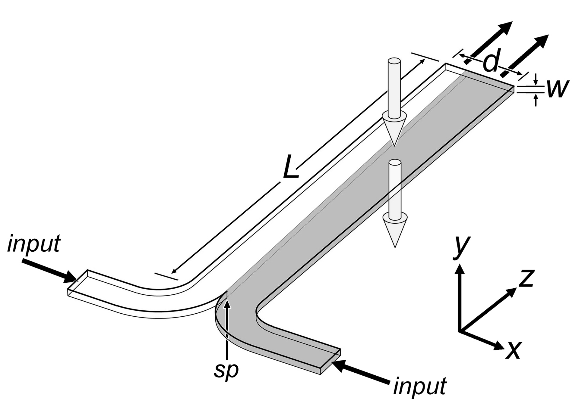
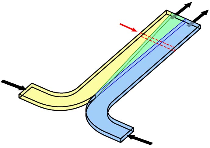
The T-Sensor in its simplest embodiment has two input ports and one outlet port, allowing two fluids to be brought into contact such that they flow side by side (Figure 2). Assuming a rectangular cross section, the relevant dimensions are the length, L, the diffusion dimension of the channel, d, and the width of the channel, w. The d-dimension is typically the larger of the two dimensions and can range anywhere from 20 to 5000 µm. The w-dimension commonly ranges from 5 to 100 µm. These dimensions produce aspect ratios, d/w, between 1 and 1000. Due to characteristics of the velocity profile within a microchannel, high aspect ratio devices are required to accurately monitor diffusion of analytes across the d-dimension without resort to the use of a complex model to interpret the data. The two fluids meet at the stagnation point (sp), an area where the local fluid velocity is near zero due to the no-slip boundary condition enforced at the walls. The stagnation point and flow development features have significant but manageable effects on downstream measurements in the T-Sensor.

Figure 2. Conceptual rendering of the operation of the T-sensor. Two fluids enter through input channels, merging at the stagnation point (sp). In the case shown here, the fluid on the right contains a diffusable analyte (gray) that spreads across the d-dimension as flow proceeds along the channel length. Typical measurements are made by fluorescence detection along the optical axis, denoted with large arrows in the y-direction.

For most applications, the diffusion and/or chemical binding of specific analytes across the d-dimensions is monitored using fluorescent indicator molecules. Upon a specific chemical binding event, these molecules experience a change in their quantum efficiency, the ratio of the number of photons incident on the molecule to the number of photons emitted (at a higher wavelength) by the molecule. By illuminating the channel with excitation light of specific wavelengths and filtering emitted light at appropriate wavelengths, digital images of the fluorescence within the channel can be captured using microscope optics and a CCD camera. In this case, the optical axis for microchannel experiments is as shown in Figure 2.

In a typical T-sensor assay, for example, one input stream contains an analyte of interest, such as a protein or a drug. The other fluid stream contains a receptor molecule such as a fluorescent indicator, an antibody, a pH indicator, an enzyme, or some other reactive species. Because the Reynolds number is small, usually much less than 1, the flow of the two streams is completely laminar and no convective mixing between the streams occurs. Thus, the only means by which molecules in opposite streams can mix is by molecular diffusion across the interface of the two fluid streams. The chemical binding or other reaction events than occur along this centerline produce a measurable signal, usually fluorescence, which can be used to calculate a parameter of interest for the analyte, such as concentration or diffusion coefficient.

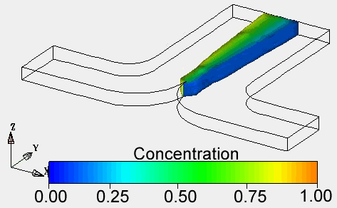
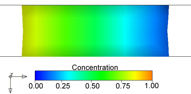
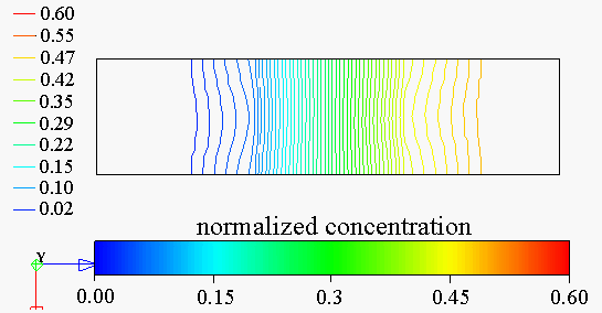
We have made extensive use of 2D models to describe mass transport in microchannels. One of the significant limitations of using a 2D model for mass transport simulations is the fact that the velocity profile will be different when also enforcing boundary conditions on the top and bottom walls. As shown in the H-filter section, the true 3D velocity profile through a channel is parabolic in both the d-dimension and the w-dimension. Figure 3 shows the true 3-D solution for the diffusion of albumin in a channel similar to those above. The flow velocity at each inlet was 100 µm/s. The maximal and minimal mass fraction values are cut away to show only the interdiffusion zone. Figures 3 and 4 also show cross-sections of this zone taken at the outlet of the channel. This view demonstrates the nonuniformity of the concentration profile due to the parabolic velocity profile. The phenomena, sometimes called the "butterfly effect," 1 is the result of the fact that the residence time is longer near the walls, allowing more diffusion to occur near the walls than in the center of the channel. Note in Figure 4 that the degree of curvature of each contour line is not the same. This is due to the fact that the parabolic velocity profile creates secondary concentration gradients across the w-dimension of the channel, resulting in different effective diffusive scaling laws for mass transport occurring in the center versus mass transport occurring near the walls. As with normal diffusion, the diffusive scaling law near the center of the channel follows a _ relationship between distance and time. However, near the walls diffusion has been shown theoretically and experimentally to follow a 1/3 power law. This nonuniformity in the concentration profile has been described in detail elsewhere.

Figure 3. The 3D interdiffusion zone for albumin (D = 65µm2/s) with inlet flow rates of 100 µm/s (left). A normalized concentration of albumin enters at the left inlet and buffer enters at the right inlet. A cross section of the concentration at the outlet of the device is shown that demonstrates the nonuniformity in the concentration profile due to parabolic flow (right).

Figure 4. Contour plot of the concentration across the outlet of the T-Sensor shown above. In this case, a normalized concentration of 0.5 initially occupies the right half of the channel.

Flow Development and Entry Length

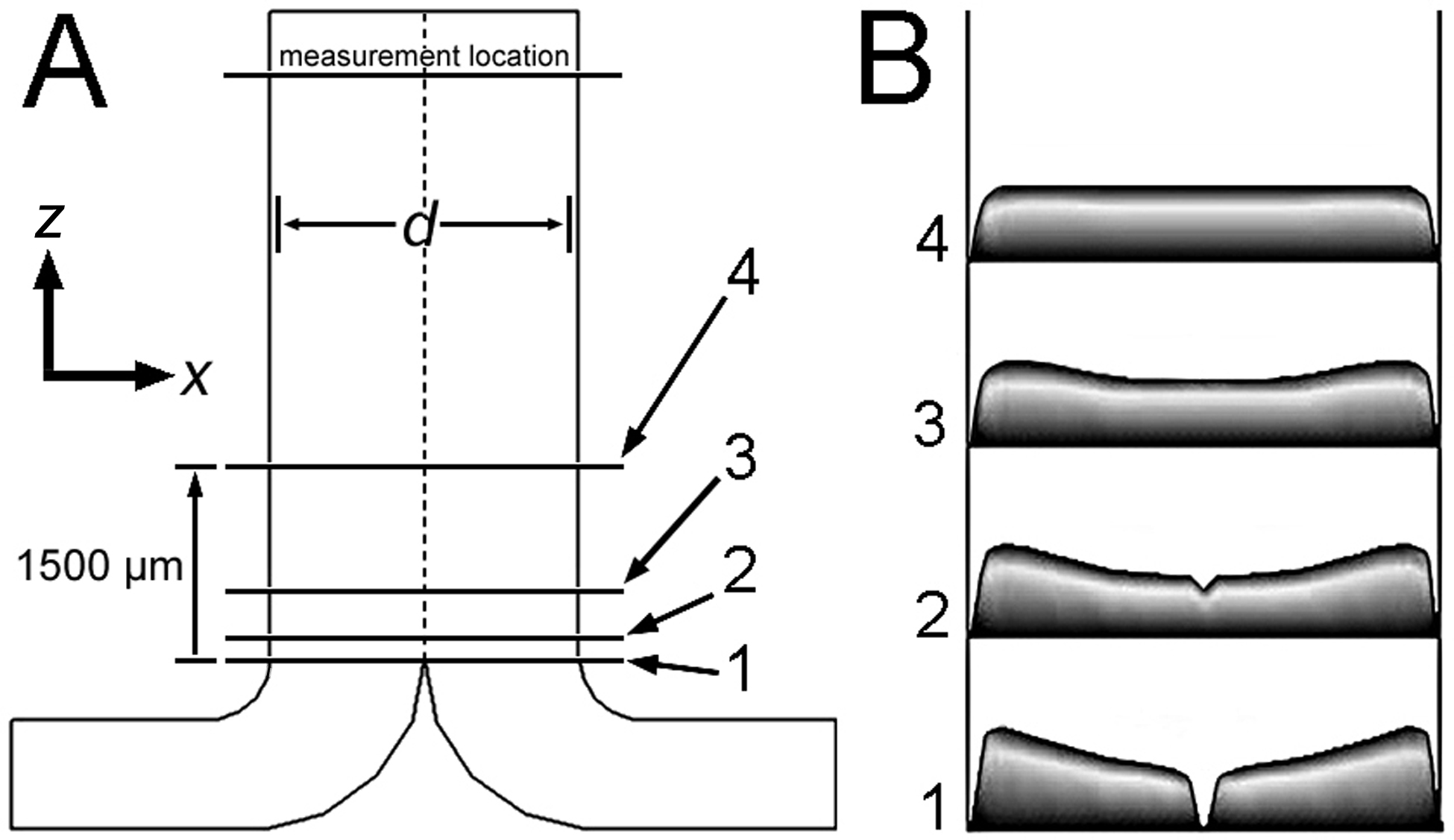
Another consideration is that of flow development, in which a finite distance is required at the entry of a channel for the velocity profile to reach a steady, fully developed state. This distance is called the entry length. Full three-dimensional numerical simulations of a typical T-Sensor geometry (d = 2405 mm, w = 10 mm) yielded the shape of the flow development region (Figure 5). Because the velocity profiles within each inlet leg are parabolic, the velocity along the centerline is zero at the stagnation point and undergoes acceleration until the flow is fully developed. Using total volumetric flow rate boundary conditions of 41.67, 500, and 1000 nl/s, all simulated velocity profiles had the same shape and relative magnitudes. Values of the velocity field were recovered from the simulations in order to determine flow development entry lengths. The distance to 95% of fully developed flow was 863.7 ± 1.5 mm, whereas that to 99% of fully developed flow was 1423 ± 5 mm. The small standard deviation in these numbers suggests that entry length is essentially independent of flow rate in the range studied.

Figure 5. Three-dimensional finite element simulations of the velocity profile development in a typical T-sensor (d = 2405 mm, w = 10 mm). For the four numbered locations marked in A, velocity profiles at the 1/2 w plane are shown in B.

Many aspects of the flow in a T-sensor with such a high aspect ratio can be treated as if the geometry is analogous to flow between infinite parallel plates. Most notably, the effective hydrodynamic length parameter used in many calculations reduces to the value of w. However, the values for entry length predicted by the three-dimensional model are not consistent with predictions of traditional fluid mechanics rules of thumb. This is due to the influence of the velocity profiles within the inlet legs on the development of the velocity along the main channel centerline. Therefore, the entry length should be dependent also on the size of the d-dimension and the geometry of the merge between the input legs.

Because the assumption that a fully developed velocity profile exists at all times in the channel is not correct, there is a potential source of error in the calculation of diffusion coefficients. Diffusion coefficients are measured experimentally by fitting the diffusion curves obtained in a T-sensor at a certain distance downstream to diffusion curves generated by a numerical model. However, this numerical model does not account for higher dimensional effects such as flow development.

To quantify the effect of flow development on diffusion coefficient measurements, three-dimensional mass transport simulations were performed using the NetFlow module of FlumeCAD. The results were compared with the results of one-dimensional model simulations that assumed the flow was fully developed throughout the channel. Because the one-dimensional model does not account for the low velocities in the flow development region, it underpredicts the residence time for molecules traveling on the centerline. This error can be quantified by comparing the residence time for a hypothetical non-diffusing particle traveling along the center-centerline in the simplified one-dimensional model and the realistic three-dimensional simulations. At a distance of 5000 mm downstream and flow rates of 42, 500 and 1000 nl/s, the one-dimensional model was found to underpredict the residence time by 29.0 ± 2.2%, which results in an overprediction of the diffusion coefficient by the same percentage. This represents the worst-case scenario because for any diffusable analyte the actual error is much less since the fluid velocities adjacent to the centerline develop much more quickly. At a distance across d of 100 mm from the centerline, the residence time underprediction falls to 9%, and at 175 mm, it is only 4%. Since the analytes used in practice undergo substantial diffusion across the d-dimension, the estimated error from entry effects is less than 5%. Therefore, while the development of flow may have a significant effect on the residence time of particles remaining exactly along the centerline, for the purposes of diffusion based experiments where no single molecule remains along the centerline for very long and measurements are made a long distance downstream of the stagnation point, entry effects are usually insignificant.

Over the last 5 years T-sensor assay feasibility has been demonstrated for a variety of clinical parameters such as blood pH and oxygen, electrolytes, proteins, enzymes and drugs, by using detection methods ranging from fluorescence and absorption to voltammetry. T-sensors measurements have been demonstrated for analytes directly in whole blood, without prior separation of blood cells. In addition, monitoring signal intensities along the T-sensor detection channel (in flow direction) provides a means of measuring the kinetics of a reaction, thus allowing kinetic diagnostic reactions to be measured not as a function of time but of distance from the starting point of interdiffusion.