Basic Microfluidic Concepts

A microfluidic device can be identified by the fact that it has one or more channels with at least one dimension less than 1 mm. Common fluids used in microfluidic devices include whole blood samples, bacterial cell suspensions, protein or antibody solutions and various buffers. Microfluidic devices can be used to obtain a variety of interesting measurements including molecular diffusion coefficients [1,2], fluid viscosity [3], pH [4,5], chemical binding coefficients [1] and enzyme reaction kinetics [6-8}. Other applications for microfluidic devices include capillary electrophoresis [9], isoelectric focusing [5,10,11], immunoassays [12-15], flow cytometry [16], sample injection of proteins for analysis via mass spectrometry [17-19], PCR amplification [20-22], DNA analysis [23-26], cell manipulation [27], cell separation [28], cell patterning [29,30] and chemical gradient formation [31,32]. Many of these applications have utility for clinical diagnostics [33,34].

The use of microfluidic devices to conduct biomedical research and create clinically useful technologies has a number of significant advantages. First, because the volume of fluids within these channels is very small, usually several nanoliters, the amount of reagents and analytes used is quite small. This is especially significant for expensive reagents. The fabrications techniques used to construct microfluidic devices, discussed in more depth later, are relatively inexpensive and are very amenable both to highly elaborate, multiplexed devices and also to mass production. In a manner similar to that for microelectronics, microfluidic technologies enable the fabrication of highly integrated devices for performing several different functions on the same substrate chip. One of the long term goals in the field of microfluidics is to create integrated, portable clinical diagnostic devices for home and bedside use, thereby eliminating time consuming laboratory analysis procedures.

Basic Principles of Microfluidics

The flow of a fluid through a microfluidic channel can be characterized by the Reynolds number, defined as

equation 1

where L is the most relevant length scale, µ is the viscosity, r is the fluid density, and V_avg is the average velocity of the flow. For many microchannels, L is equal to 4A/P where A is the cross sectional area of the channel and P is the wetted perimeter of the channel. Due to the small dimensions of microchannels, the Re is usually much less than 100, often less than 1.0. In this Reynolds number regime, flow is completely laminar and no turbulence occurs. The transition to turbulent flow generally occurs in the range of Reynolds number 2000. Laminar flow provides a means by which molecules can be transported in a relatively predictable manner through microchannels. Note, however, that even at Reynolds numbers below 100, it is possible to have momentum-based phenomena such as as flow separation.

Pressure Driven Flow

There are two common methods by which fluid actuation through microchannels can be achieved. In pressure driven flow, in which the fluid is pumped through the device via positive displacement pumps, such as syringe pumps. One of the basic laws of fluid mechanics for pressure driven laminar flow, the so-called no-slip boundary condition, states that the fluid velocity at the walls must be zero. This produces a parabolic velocity profile within the channel (Figure 1.1).

As discussed in Chapter 2, the parabolic velocity profile has significant implications for the distribution of molecules transported within a channel. Pressure driven flow can be a relative inexpensive and quite reproducible approach to pumping fluids through microdevices. With the increasing efforts at developing functional micropumps, pressure driven flow is also amenable to miniaturization.

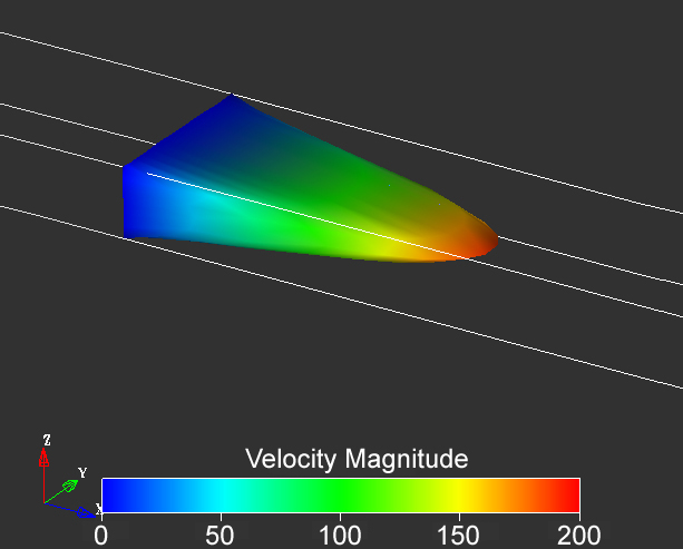
Figure 1.1. Velocity profile in a microchannel with aspect ratio 2:5 under conditions of pressure driven flow. Note that the velocity is assumed to be zero at the walls in most treatments of transport of liquids. Image from result of a calculation using Coventorware software.

Electrokinetic Flow

Another common technique for pumping fluids is that of electroösmotic pumping. If the walls of a microchannel have an electric charge, as most surfaces do, an electric double layer of counter ions will form at the walls. When an electric field is applied across the channel, the ions in the double layer move towards the electrode of opposite polarity. This creates motion of the fluid near the walls and transfers via viscous forces into convective motion of the bulk fluid. If the channel is open at the electrodes, as is most often the case, the velocity profile is uniform across the entire width of the channel (Figure 1.2). However, if the electric field is applied across a closed channel (or a backpressure exists that just counters that produced by the pump), a recirculation pattern forms in which fluid along the center of the channel moves in a direction opposite to that at the walls (Figure 1.3). In closed channels, the velocity along the centerline of the channel is 50% of the velocity at the walls.

Figure 1.2. The very uninteresting flow velocity profile calculated for electroösmotic pumping in an open channel. Such a channel (in the absence of backpressure) exhibits plug flow. Shown in the situation for negatively charged walls; the anode is at the left and the cathode is at the right. In fact the profile is very interesting close to the walls, since velocity drops to zero at the walls over a distance that is comparable to the thickness of the electrical double layer.

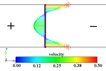
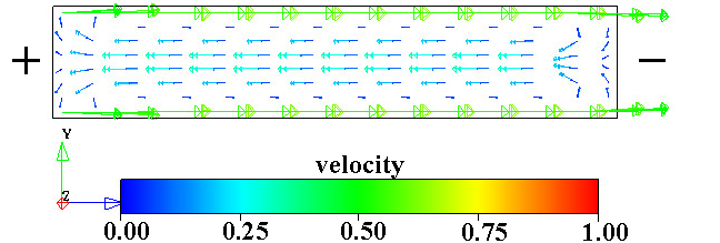
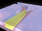
Figure 1.3. Two views of the electroösmotic flow velocity vectors in a closed channel. Note that the recirculation results in equal total flows to the right and left at all vertical planes through the channel. In both images the anode is on the left and the cathode is on the right and the walls are negatively charged. Images from results of calculations using Coventorware software.

One of the advantages of electrokinetic flow is that the blunt velocity profile avoids many of the diffusion nonuniformities that occur with pressure driven flow. However, sample dispersion in the form of band broadening is still a concern for electroösmotic pumping. Another advantage to electrokinetic flow is that it is straight forward to couple other electronic applications on-chip. However, electrokinetic flow often requires very high voltages, making it a difficult technology to miniaturize without off-chip power supplies. Another significant disadvantage of electrokinetic flow is the variability in surface properties. Proteins, for example, can adsorb to the walls, substantially change the surface charge characteristics and, thereby, change the fluid velocity. This can result in unpredictable long-term time dependencies in the fluid flow.

Introduction to Finite Element Modeling in Fluid Mechanics

The Utility of Modeling

Because the field of microfluidics is a relatively immature field, numerical simulations of microfluidic systems can be extremely valuable both in terms of providing a research tool and as an efficient design and optimization tool. By incorporating the complexities of channel geometry, fluid flow rates, diffusion coefficients and possible chemical interactions into a numerical model, the behavior of a particular system can be accurately predicted when an intuitive prediction may be extremely difficult. For example, a custom coded numerical model has been used to predict differences in the diffusive scaling laws across the depth of a microchannel. Numerical modeling also allows visualization of complex flow phenomena that may not be easily obtained experimentally.

However, perhaps the greatest use of numerical modeling, particular in the form of a convenient commercially available package, is as a design tool. In this case, the model can be used to explore the effects of changing any number of parameters on the performance of the device without actually fabricating different devices. For example, different channel geometries can be simulated to explore the extent of interdiffusion or chemical binding along the centerline of a T-Sensor to determine the parameters required for a desired diffusion profile.

The weakness of numerical modeling is, of course, the fact that it is not guaranteed to exactly replicate events in nature, particularly if there are physical phenomena that are not incorporated into the model. Because of the numerical approximations required by the finite element method (see below), there is also the danger of slightly inaccurate simulation results. However, careful examination of simulation results and comparison of numerical and experimental data can validate the use of the model as a predictive tool. The commercial modeling package used in this research has been shown to be reasonably accurate, both from comparisons with experimentally obtained images and from comparison with a different numerical modeling approach. These features will be described in more detail below.

Governing Equations in Fluid Mechanics

The flow of fluid through a control volume can be described by the complete Navier-Stokes equations. These equations can be derived from the principles of conservation of mass, momentum and energy. The conservation of mass equation states that at all times (for incompressible, steady flow) the mass entering the control volume is equal to the mass leaving the control volume,

equation 2

where Á is the fluid density, t is time and v is the local fluid velocity. This equation is also often called the 'continuity equation' because it is based on the assumption that the fluid medium is continuous. The continuity approximation is valid when the Knudsen number, the ratio of the mean free path of the fluid, », to the length scale of the system, L,

equation 3

is less than 0.3. For most fluids, including water, the continuity approximation is nearly always valid.

As an analog to Newton's second law of motion, the conservation of momentum equation states that the change in momentum within the control volume is equal to the sum of the forces acting on the control volume,

equation 4

where P is the pressure, Ä is the viscous stress, g is the gravitational body force and F is any other body force.

The energy equation is essentially a statement of the first law of thermodynamics: the energy within a region, due to work and heat transfer, is constant,

equation 5

Here, µ is the internal energy of the system, k is the thermal conductivity of the fluid, H is an energy source term and X is an energy dissipation term. In general, the energy equation is coupled with the continuity and momentum equations due to the variation in density with pressure and temperature. However, for the cases of incompressible flow such that the density variation is negligible, the energy equation can be decoupled from the mass and momentum equations.

The Finite Element Method

Although there are several methods for spatially discretizing differential equations over a solution domain, such as the finite difference and finite volume methods, a common method for solving fluidics problems is the finite element method. For any system of ordinary differential equations (linear or nonlinear), the finite element method can be summarized as follows. First, the solution domain is spatially discretized by constructing a series of interlocking nodes and elements, resulting in a finite number of elements that approximate the spatial geometry. These elements can have a number of shapes including linear, triangular and parabolic. Using techniques in variational calculus, the variational form, or the 'functional,' that satisfies the specified partial differential equation is constructed. Next, an approximation for the field is introduced by matrix multiplying linear basis functions by unknown nodal values. The approximation is then inserted into the functional and the functional is minimized, a process that is equivalent to minimizing the error function of the equation. This minimization is achieved when the functional is a set of nonlinear algebraic equations of the form,

KU = F, [6]

where K is the global system matrix, or the 'stiffness' matrix, U is the global matrix of unknowns (velocities, pressures, etc.) and F, the 'force' matrix, contains effects of all relevant body forces and boundary conditions. Solving this matrix equation results in a solution for the computational domain at the nodes with, in the case of linear elements, linear interpolation between nodes.

References:

1.Kamholz, A. E., Weigl, B. H., Finlayson, B. A. & Yager, P. Quantitative analysis of molecular interaction in a microfluidic channel: The T-sensor. Analytical Chemistry 71, 5340-5347 (1999).

2.Kamholz, A. E., Schilling, E. A. & Yager, P. Optical measurement of transverse molecular diffusion in a microchannel. Biophysical Journal 80, 1967-1972 (2001).

3.Galambos, P. Ph.D. Thesis, Mechanical Engineering. University of Washington, Seattle (1998).

4.Weigl, B. H. & Yager, P. Silicon-microfabricated diffusion-based optical chemical sensor. Sensors and Actuators B-Chemical 39, 452-457 (1997).

5.Macounova, K., Cabrera, C. R., Holl, M. R. & Yager, P. Generation of natural pH gradients in microfluidic channels for use in isoelectric focusing. Analytical Chemistry 72, 3745-3751 (2000).

6.Hadd, A. G., Raymond, D. E., Halliwell, J. W., Jacobson, S. C. & Ramsey, J. M. Microchip device for performing enzyme assays. Analytical Chemistry 69, 3407-3412 (1997).

7.Duffy, D. C., Gillis, H. L., Lin, J., Sheppard, N. F. & Kellogg, G. J. Microfabricated centrifugal microfluidic systems: Characterization and multiple enzymatic assays. Analytical Chemistry 71, 4669-4678 (1999).

8.Hadd, A. G., Jacobson, S. C. & Ramsey, J. M. Microfluidic assays of acetylcholinesterase inhibitors. Analytical Chemistry 71, 5206-5212 (1999).

9.Kameoka, J., Craighead, H. G., Zhang, H. W. & Henion, J. A polymeric microfluidic chip for CE/MS determination of small molecules. Analytical Chemistry 73, 1935-1941 (2001).

10.Xu, J., Lee, C. S. & Locascio, L. E. Isoelectric focusing of green fluorescence proteins in plastic microfluid channels. Abstracts of Papers of the American Chemical Society 219, 9-ANYL (2000).

11.Macounova, K., Cabrera, C. R. & Yager, P. Concentration and separation of proteins in microfluidic channels on the basis of transverse IEF. Analytical Chemistry 73, 1627-1633 (2001).

12.Hatch, A. et al. A rapid diffusion immunoassay in a T-sensor. Nature Biotechnology 19, 461-465 (2001).

13.Eteshola, E. & Leckband, D. Development and characterization of an ELISA assay in PDMS microfluidic channels. Sensors and Actuators B-Chemical 72, 129-133 (2001).

14.Cheng, S. B. et al. Development of a multichannel microfluidic analysis system employing affinity capillary electrophoresis for immunoassay. Analytical Chemistry 73, 1472-1479 (2001).

15.Yang, T. L., Jung, S. Y., Mao, H. B. & Cremer, P. S. Fabrication of phospholipid bilayer-coated microchannels for on-chip immunoassays. Analytical Chemistry 73, 165-169 (2001).

16.Sohn, L. L. et al. Capacitance cytometry: Measuring biological cells one by one. Proceedings of the National Academy of Sciences of the United States of America 97, 10687-10690 (2000).

17.Figeys, D., Gygi, S. P., McKinnon, G. & Aebersold, R. An integrated microfluidics tandem mass spectrometry system for automated protein analysis. Analytical Chemistry 70, 3728-3734 (1998).

18.Jiang, Y., Wang, P. C., Locascio, L. E. & Lee, C. S. Integrated plastic microftuidic devices with ESI-MS for drug screening and residue analysis. Analytical Chemistry 73, 2048-2053 (2001).

19.Gao, J., Xu, J. D., Locascio, L. E. & Lee, C. S. Integrated microfluidic system enabling protein digestion, peptide separation, and protein identification. Analytical Chemistry 73, 2648-2655 (2001).

20.Belgrader, P., Okuzumi, M., Pourahmadi, F., Borkholder, D. A. & Northrup, M. A. A microfluidic cartridge to prepare spores for PCR analysis. Biosensors & Bioelectronics 14, 849-852 (2000).

21.Khandurina, J. et al. Integrated system for rapid PCR-based DNA analysis in microfluidic devices. Analytical Chemistry 72, 2995-3000 (2000).

22.Lagally, E. T., Medintz, I. & Mathies, R. A. Single-molecule DNA amplification and analysis in an integrated microfluidic device. Analytical Chemistry 73, 565-570 (2001).

23.Buchholz, B. A. et al. Microchannel DNA sequencing matrices with a thermally controlled "viscosity switch". Analytical Chemistry 73, 157-164 (2001).

24.Fan, Z. H. et al. Dynamic DNA hybridization on a chip using paramagnetic beads. Analytical Chemistry 71, 4851-4859 (1999).

25.Koutny, L. et al. Eight hundred base sequencing in a microfabricated electrophoretic device. Analytical Chemistry 72, 3388-3391 (2000).

26.Lee, G. B., Chen, S. H., Huang, G. R., Sung, W. C. & Lin, Y. H. Microfabricated plastic chips by hot embossing methods and their applications for DNA separation and detection. Sensors and Actuators B-Chemical 75, 142-148 (2001).

27.Glasgow, I. K. et al. Handling individual mammalian embryos using microfluidics. Ieee Transactions On Biomedical Engineering 48, 570-578 (2001).

28.Yang, J., Huang, Y., Wang, X. B., Becker, F. F. & Gascoyne, P. R. C. Cell separation on microfabricated electrodes using dielectrophoretic/gravitational field flow fractionation. Analytical Chemistry 71, 911-918 (1999).

29.Chiu, D. T. et al. Patterned deposition of cells and proteins onto surfaces by using three-dimensional microfluidic systems. Proceedings of the National Academy of Sciences of the United States of America 97, 2408-2413 (2000).

30.Folch, A., Jo, B. H., Hurtado, O., Beebe, D. J. & Toner, M. Microfabricated elastomeric stencils for micropatterning cell cultures. Journal of Biomedical Materials Research 52, 346-353 (2000).

31.Dertinger, S. K. W., Chiu, D. T., Jeon, N. L. & Whitesides, G. M. Generation of gradients having complex shapes using microfluidic networks. Analytical Chemistry 73, 1240-1246 (2001).

32.Jeon, N. L. et al. Generation of solution and surface gradients using microfluidic systems. Langmuir 16, 8311-8316 (2000).

33.Weigl, B. H. & Yager, P. Microfluidics - Microfluidic diffusion-based separation and detection. Science 283, 346-347 (1999).

34.Cunningham, D. D. Fluidics and sample handling in clinical chemical analysis. Analytica Chimica Acta 429, 1-18 (2001).

We recognize that the content of these pages is extremely basic. Several excellent texts on fluidics exist, and there are numerous recent recent research articles that are useful. As useful material appears on the web, we will provide links. If you know of useful material that can be liked, please send Yager the URL.