Lab 0
Contents
Preliminaries
The lab section of this course gives an opportunity to implement the ideas that come from lecture. Numerical analysis allows one to experiment directly with ideas from calculus, linear algebra and beyond.
The grade for this lab section is based on weekly homework assignments assigned in lecture (50%) and a final project (50%). Not all homework assignments will have a lab assignment.
Homework is due at the end of the day the Thursday after it is assigned. We will take lab time to work on the assignments. Late assignments will not be accepted.
The project will assigned early in the quarter and will be due at the end of the day on Dec. 8. It will consist of an in-depth coding project.
In this class we will use the "publish" functionality of MATLAB® extensively. All MATLAB work that is turned it should be written so that it is readable after "publishing it". Please see me or the TA if you have any questions about this functionality. Here is the official documentation for publishing: Publishing Markup
MATLAB® Links
UCI MATLAB Software Installation
Some other references for MATLAB® tutorials are:
Some basic commands
clear % clear workspace
1 + 1
sin(pi*3)
exp(-1)
tanh(20)
ans =

     2


ans =

   3.6739e-16


ans =

    0.3679


ans =

     1
Defining vectors
v = [1 2 3]; % a row vector, semi-colon supresses output
w = [1; 2; 3]; % a column vector
v - w' %' gives the transpose
ans =

     0     0     0
Long vectors
v = [1:9] % a vector of integers 1 through 9
v(1) % first element of v
v(end) % last element of v
v(2:7) % grab elements 2 through 7
v(4:end) % grab elements 4 through the end
v =

     1     2     3     4     5     6     7     8     9


ans =

     1


ans =

     9


ans =

     2     3     4     5     6     7


ans =

     4     5     6     7     8     9
Matrices
M = [1,2,3,4;5,6,7,8;9,10,11,12;12,14,15,16]
M(1,4) % get the (1,4) element
M(2:3,2:3) % get the "middle" block of the matrix
M =

     1     2     3     4
     5     6     7     8
     9    10    11    12
    12    14    15    16


ans =

     4


ans =

     6     7
    10    11
Plotting
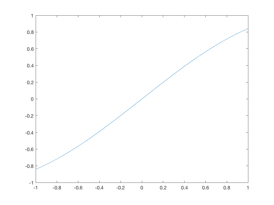
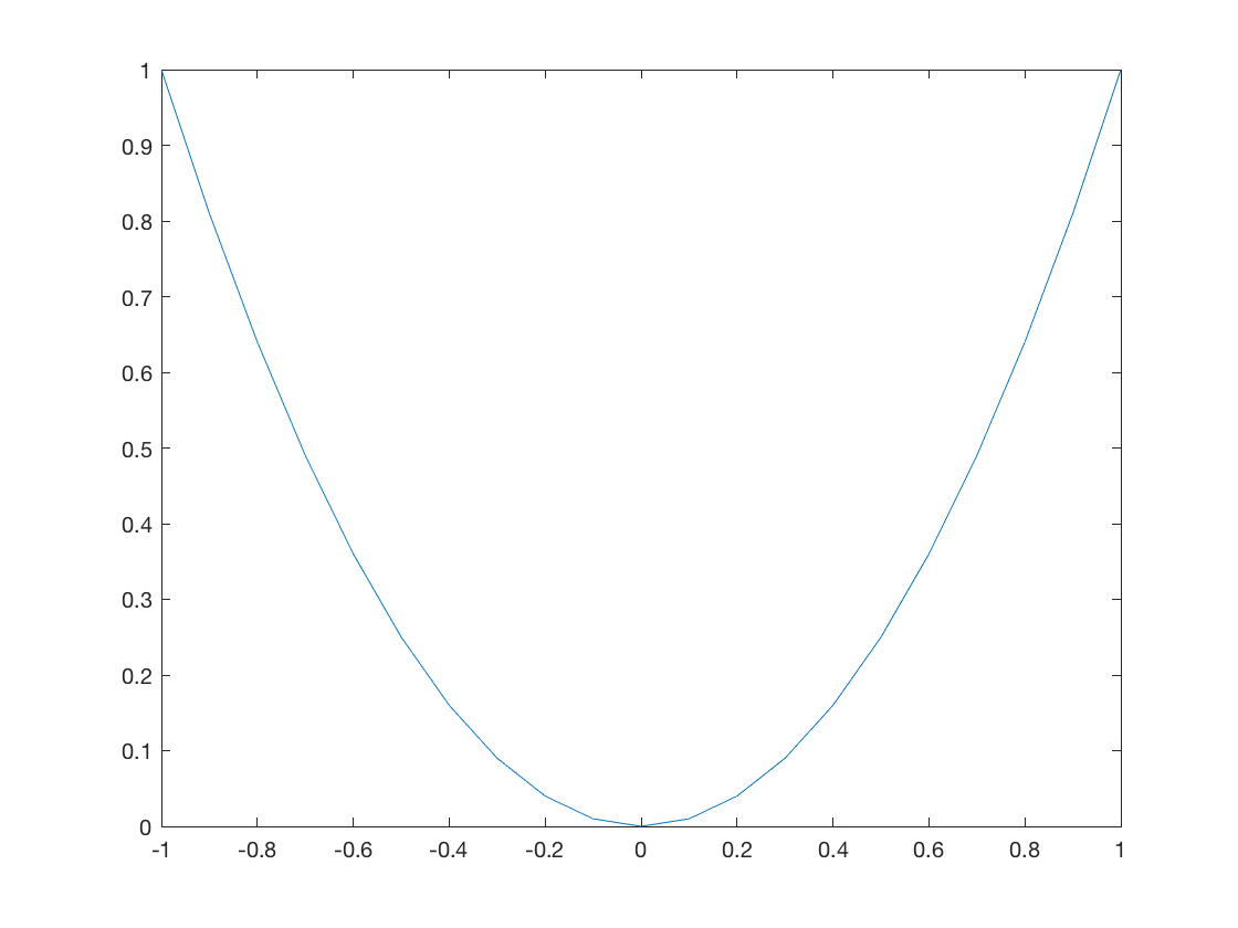
x = linspace(-1,1,100); % use 100 points between -1 and 1;
y = sin(x);
figure(1) % select a figure
plot(x,y)

x = -1:.1:1; % points from -1 to 1 with a spacing of .1;
y = x.^2; % use .^ or .* or ./ apply this operations to vectors componentwise
figure(2)
plot(x,y)
Plotting two functions with labels
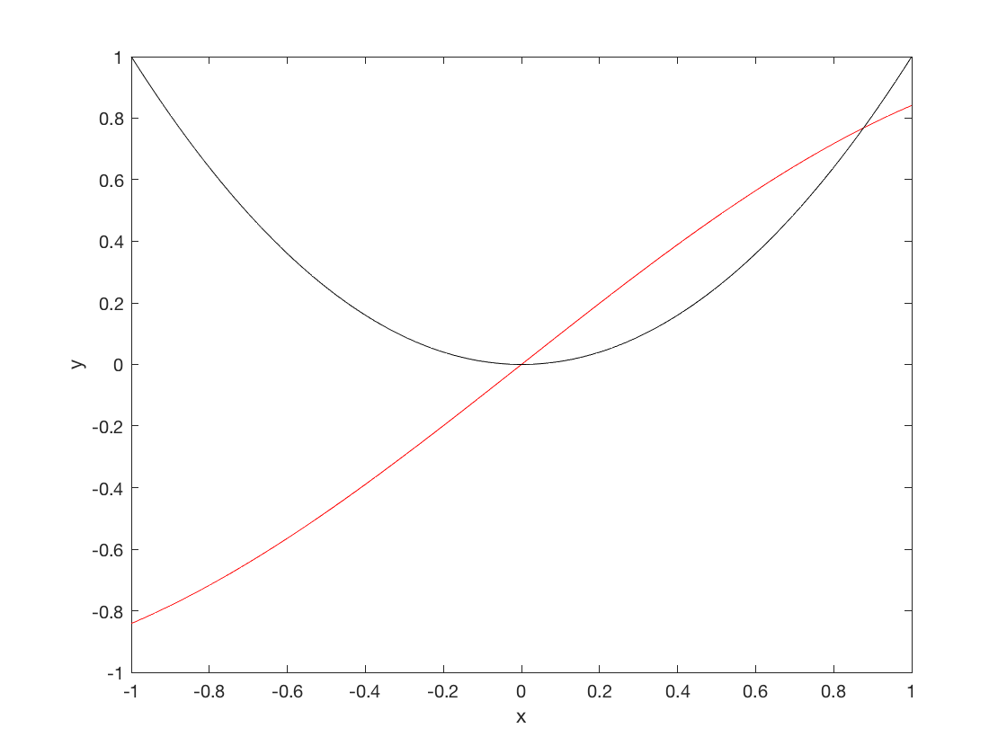
x = linspace(-1,1,100);
figure(3)
plot(x,sin(x),'r') % plot in red
hold on % prevent the figure from being overwitten
plot(x,x.^2,'k') % plot in black
xlabel('x')
ylabel('y')
for loops (notice the tab's for text alignment)
The following should give the sum of the first  integers which is
n = 10;
SUM = 0; % using capital letters because sum() is a built-in function
for i = 1:n
    SUM = SUM + i;
end
SUM
n*(n+1)/2
SUM =

    55


ans =

    55
a function
We can define anonymous functions in this way:
g = @(n) sum([0:n]);
g(10)
ans =

    55
Problem 1:
Define
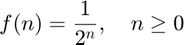
Write code to plot the two functions  and
and  for
for  . The command
plot(x,y,'*')
will plot the function but not interpolate between data points. Hint: look at the
cumsum()
command.
Problem 2:
Define the matrix
![$$ M = \left[ \begin{array}{ccc} 1 & 2 & 1 \\ 2 & 4 & 3 \end{array} \right].$$](Lab0_eq17410629534189950302.png)
Write code to subtract twice the first row from the second.