These functions provide a basic level of support for categorical predictor variables to be used in the Lisp-Stat regression functions. You can use just these to get more control over the process. After writing all the formula methods I found out that there were already primitive functions like this provided with glim-proto.
There are three main functions: (factor), (interaction), and (block-test). The first constructs a set of treatment contrasts -- indicator variables for all but the first level of the factor -- and optionally a set of appropriate names. The second takes a list of variables and constructs a matrix of variables for the interaction terms. It allows both continuous and factor variables. Only the highest order interaction terms are included, so to get a matrix for the model 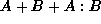 you would need to call (factor) on each of A and B and then (interaction) on A and B together. This behaviour is useful for two reasons: it makes it much easier to implement a model formula system and it allows non-hierarchical models on the occasions when they are appropriate. The third function calculates and displays the Wald test for a block of variables all having zero coefficient and the individual coefficient estimates, standard errors and Wald p-values.
There are also two functions (design) and (names) that return the design matrix or list of names from a list of terms of the sort returned by (factor) and (interaction).
(factor x &key namebase).
x is a sequence and namebase is either a string or a symbol. Returns a list containing the design matrix of treatment contrasts and a list of variable names. If namebase is nil returns only the design matrix ( not a list containing only the design matrix)
>(factor (list 2 3 4 2 3 4) :namebase "A")
(#2A((0 0) (1 0) (0 1) (0 0) (1 0) (0 1)) ("(A 3)" "(A 4)"))

>(factor (list 2 3 4 2 3 4) :namebase 'A)
(#2A((0 0) (1 0) (0 1) (0 0) (1 0) (0 1)) ("(A 3)" "(A 4)"))

> (factor (list 2 3 4 2 3 4) )
#2A((0 0) (1 0) (0 1) (0 0) (1 0) (0 1))
(interaction (xs &key (is-factor (repeat t (length xs))) (namebases (repeat nil (length xs))) )
xs is a list of sequences, is-factor is a list of t and nil values indicating whether the respective variable should be treated as a factor, namebases is a list of strings or symbols. Returns a design matrix (if namebases or (first namebases) is nil) or a list containing a design matrix and a list of names.
> (def a (list 1 2 1 2 1 2))
A
> (def b (list 5 6 7 5 6 7))
B
> (def c (list 0.1 0.2 0.3 0.4 0.5 0.6))
C
> (interaction (list a b) :is-factor (list t t) :namebases (list "A" 'B))
(#2A((0 0) (1 0) (0 0) (0 0) (0 0) (0 1)) ("((A 2) (B 6))" "((A 2) (B 7))"))
> (interaction (list a c) :is-factor (list t nil) :namebases (list "A" "C"))
(#2A((0.0) (0.2) (0.0) (0.4) (0.0) (0.6)) ("((A 2) C)"))
> (interaction (list a b c) :is-factor (list t t  nil)
:namebases (list "A" "B" "C"))
(#2A((0.0 0.0) (0.2 0.0) (0.0 0.0) (0.0 0.0) (0.0 0.0) (0.0 0.6))
 ("(((A 2) (B 6)) C)" "(((A 2) (B 7)) C)"))
>  (interaction (list a b c) :is-factor (list t t  nil) )
#2A((0.0 0.0) (0.2 0.0) (0.0 0.0) (0.0 0.0) (0.0 0.0) (0.0 0.6))
(block-test (index beta covmat &key blockname names (block-only nil))
index is a sequence of integers indicating which components of the coefficient vector are in the block, beta is the coefficient vector, covmat is the covariance matrix, blockname is a string giving the name of the block as a whole. Prints out a table with the Wald test of the hypothesis that all the coefficients in the block are zero and if block-only is nil separate tests for each coefficient.
> (def a (binomial-rand 100 4 0.3))
A
> (def b (binomial-rand 100 4 0.3))
B
> (def x (normal-rand 100 ))
X
> (def y (+ a x (normal-rand 100)))
Y
> (def factora (factor b :namebase "B"))
FACTORA
> (def factora (factor a :namebase "A"))
FACTORA
> (def factorb (factor b :namebase "B"))
FACTORB
> (def varx (list x '("X")))
VARX
> (def ab (interaction (list a b) :namebases (list "A" "B")))
AB
> (def ax (interaction (list a x) :namebases (list "A" "X")
:is-factor (list t nil)))
AX
> (def bx (interaction (list b x) :namebases (list "B" "X")
:is-factor (list t nil)))
BX
> (def abx (interaction (list a b x) :namebases (list "A" "B" "X")
:is-factor (list t t nil)))
ABX
> (def model1 (regression-model (design (list factora varx)) y
:predictor-names (names (list factora varx))))

Least Squares Estimates:

Constant                  0.299999      (0.200000)
(A 1)                     0.677777      (0.255555)
(A 2)                      1.74724      (0.277777)
(A 3)                      2.61529      (0.388888)
(A 4)                      4.33253      (0.699999)
X                          1.00357      (9.175541E-2)

R Squared:                0.700000
Sigma hat:                0.933333
Number of cases:               100
Degrees of freedom:             94

MODEL1
> (def model1-cov (* (send model1 :sigma-hat) (send model1 :xtxinv)))
MODEL1-COV

>(block-test (list 0 1 2 3) (send model1 :coef-estimates) model1-cov
:blockname "A" :names (names (list factora)) )
A                 227.13      0.0000
     (A 1)                 0.29999      (0.211111)          0.1666
     (A 2)                 0.67777      (0.266666)          0.0096
     (A 3)                  1.7472      (0.288888)          0.0000
     (A 4)                  2.6153      (0.400000)          0.0000

> (block-test (list 0 1 2 3) (send model1 :coef-estimates) model1-cov
:blockname "A" :block-only t)
A                 227.13      0.0000
>(def model2 (regression-model (design (list factora factorb  ax bx varx)) y
:predictor-names (names (list factora factorb  ax bx varx))))

Least Squares Estimates:

Constant                  -6.656751E-2  (0.266666)
(A 1)                     0.722222      (0.255555)
(A 2)                      1.75989      (0.288888)
(A 3)                      2.69490      (0.399999)
(A 4)                      4.66799      (0.699999)
(B 1)                     0.533333      (0.255555)
(B 2)                     0.155555      (0.277777)
(B 3)                     0.422222      (0.355555)
((A 1) X)                 0.233333      (0.277777)
((A 2) X)                 0.455555      (0.299999)
((A 3) X)                 0.199999      (0.388888)
((A 4) X)                  1.24579      (0.999999)
((B 1) X)                -0.288888      (0.277777)
((B 2) X)                 0.133333      (0.299999)
((B 3) X)                -0.611111      (0.399999)
X                         0.866666      (0.300000)

R Squared:                0.744444
Sigma hat:                0.900000
Number of cases:               100
Degrees of freedom:             84

MODEL2
> (def model2-cov (* (send model2 :sigma-hat ) (send model2 :xtxinv)))
MODEL2-COV
> (block-test (list 0 1 2 3) (send model2 :coef-estimates) model2-cov
:blockname "A" :block-only t)
A                 81.223      0.0000
> (block-test (list 4 5 6) (send model2 :coef-estimates) model2-cov
:blockname "B" :block-only t)
B                 45.812      0.0000
> (block-test (iseq 7 10) (send model2 :coef-estimates) model2-cov
:blockname "AX" :block-only t)
AX                3.4602      0.4888
> (block-test (iseq 11 13) (send model2 :coef-estimates) model2-cov
:blockname "BX" :block-only t)
BX                4.8578      0.1888