Deletion diagnostics are available as well as a variety of flavours of residual. Current graphical methods are
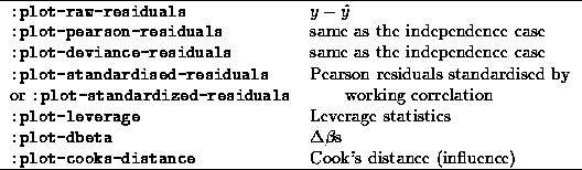
The standardised residuals are the Pearson residuals multiplied by the Cholesky square-root of the inverse of the correlation matrix. They are approximately independent with equal variance if the working model is roughly true.
The last three methods are generalisations of the leverage (diagonal of hat matrix), DBETA (change in coefficient when point is deleted) and Cook's distance (influence) statistics for linear and generalised linear models. The formulae are from Preisser & Qaqish (1996) and are natural generalisations of the independent data versions (though the derivations and calculations are rather more complicated). The methods take a keyword argument :unit of 0 for individual observation deletion and 1 for group deletion. Constants +group+ and +cluster+, and +not-group+ and +observation+ have been defined to make these easier to use (eg :unit +group+). The default is diagnostics for individual observations.
The residual plots and plot-dbeta take a keyword argument :variable. The argument for :variable is a list of indices specifying which delta-betas to plot or which variables to plot the residuals against. For :plot-dbetas variable 0 is the intercept, for :plot-...-residuals it is the linear predictor. If variable is not specified the delta-betas plot uses all variables; the residual plots just use the linear predictor. In addition, :plot-...-residuals has a :smooth keyword which indicates whether a lowess smoother should be added to the plot. The default is t for both show-labels and smooth. Any other arguments given to these functions will be passed to a call to plot-points.
The plots produced by these methods are linked, so that selections in one plot show up in the others. The residual plots also have an additional mouse mode ``group highlighting'' where selecting a point also selects all the other points in the same group. The linking is different from the usual mechanism in that all group-level plots are linked and all observation-level plots are linked but plots at different levels are not linked to each other. The gee object contains lists of observation-level and group-level plots that are separate from the linking list maintained by XLISP-Stat. To link another plot (eg a scatterplot of covariates) use the :bind-plot-to-gee message
(send mygee :bind-plot-to-gee a-plot +group+)links a-plot to the group-level plots and similarly
(send mygee :bind-plot-to-gee a-plot +observation+)links it to the observation-level diagnostic plots.
The same method names without the plot- prefix return the values of the diagnostics. The individual observation diagnostics are returned in a list or matrix in the same order as the data set; the group diagnostics have the group identifier attached and are in no reliable order. The plotting methods call two plotting functions which may be useful for other purposes: index-plot and scatter-smooth. The former takes a single argument and plots it against the integers; the second behaves like plot-points but also adds a lowess smooth to the plot.
Applying these methods to the model above, we do the following
>(send example1 :plot-dbeta)
computing diagnostic information
(#<Object: 2799672, prototype = SCATTERPLOT-PROTO> #<Object: 2771752,
prototype = SCATTERPLOT-PROTO> #<Object: 2847416, prototype =
SCATTERPLOT-PROTO> #<Object: 1545912, prototype = SCATTERPLOT-PROTO>
 #<Object: 1665112, prototype = SCATTERPLOT-PROTO> #<Object: 2305384
, prototype = SCATTERPLOT-PROTO> #<Object: 2399720, prototype =
SCATTERPLOT-PROTO>)
This gives seven plots of delta-betas showing the approximate effect on the intercept and six regression coefficients of deleting each observation. The plot titles are taken from the predictor-names argument of the model. Looking at the plot for ``smoker'' (the main variable of interest) we see that there is a large positive delta-beta value. Clicking on this point labels it as observation 15, and also highlights the other three observations on the same individual, showing that one has the largest negative delta-beta and another has a substantial positive delta-beta. Looking at the highlighting in the other plots shows that observation 15 also has large influence on the coefficent of the last time variable.
As an illustration of the plot-linking methods we produce a Normal quantile plot of residuals and link it to the other observation-level plots.
> (def resid (send example1 :deviance-residuals))
RESID
> (def qqnorm (quantile-plot resid))
QQNORM
> (send example1 :bind-plot-to-gee qqnorm +observation+)
T
When a point is selected on the individual-level delta-beta plots it and the others in the same group are now highlighted on the quantile plot. This is not very informative in these data.
As more than one of the observations on this individual is influential we examine the effect of deleting all four of her observations. In order to reduce the number of superfluous windows, only the smoking and the last time variable will be examined. These are variables 2 and 6, counting the intercept as 0.
>(send example1 :plot-dbeta :unit +group+ :variable (list 2 6))
(#<Object: 2694968, prototype = SCATTERPLOT-PROTO>
#<Object: 2724856, prototype = SCATTERPLOT-PROTO>)
These plots show individual 19 as having very strong influence on the estimated coefficient of the smoking variable. Looking at the data we find that individual 19 is the same one we previously identified. The plot shows that removing this individual from the data would increase the coefficient of the smoking variable by about .12, nearly doubling it. The effect on the time variable is also large, but proportionally much smaller and of less intrinsic interest.
Residual plots against the linear predictor are also illuminating. The following commands plot the Pearson residuals and the standardised (decorrelated) Pearson residuals against the linear predictor. Plotting against another variables is not very useful in these data as most of the variables are binary.
> (send example1 :plot-pearson-residuals :variable (list 0))
#<Object: 2688968, prototype = SCATTERPLOT-PROTO>
> (send example1 :plot-standardised-residuals :variable (list 0))
#<Object: 2731752, prototype = SCATTERPLOT-PROTO>
The largest positive Pearson residual belongs to observation 15. Its value appears very large even considering that these residuals have not been divided by the square-root of the estimated scale factor (1.35 in this case). This residual is substantially reduced when the residuals are standardised by the square-root of the working correlation matrix. The large reduction may indicate that this observation has a large influence on the correlation estimates as well as on the regression coefficients.
To examine this further we refit the model without individual 19. The Lisp-Stat commands that create the new data set are in the example file and will not be repeated here.
(def example3 (gee-model :y newy :x (list newsex newsmoke newage newtime2
 newtime3 newtime4) :g newid :error poisson-error :correlation
(stat-m-dependence 3) :times newtimes :predictor-names (list "sex"
 "smoker" "mother's age" "2nd vs 1st" "3rd vs 1st" "4th vs 1st")))
No link specified - canonical link used
Iteration 1: quasideviance = 497.561
Iteration 2: quasideviance = 448.323
Iteration 3: quasideviance = 444.118
Iteration 4: quasideviance = 444.210
Iteration 5: quasideviance = 444.265
Iteration 6: quasideviance = 444.268
Iteration 7: quasideviance = 444.268

GEE Estimates:

                         Coefficient     Std Error           Naive Std Error
Constant                  -8.675037E-2  (0.277216)          (0.365146)
sex                       -8.533069E-2  (0.188420)          (0.210624)
smoker                    0.343040      (0.216824)          (0.235934)
mother's age               6.217507E-3  (6.000891E-3)       (5.775124E-3)
2nd vs 1st               -0.462035      (0.200852)          (0.196008)
3rd vs 1st               -0.356675      (0.207296)          (0.189279)
4th vs 1st                -1.27297      (0.202666)          (0.233578)

Scale Estimate:            1.68717
Independence model deviance:   444.268
Number of cases:               288
Link:                    #<Glim Link Object: LOG-LINK>
Variance function:       Poisson error
Stationary  3 - dependence Working Model:
 correlation matrix =
#2a(
    (  1.0      0.12      0.13      0.35    )
    ( 0.12       1.0      0.12      0.13    )
    ( 0.13      0.12       1.0      0.12    )
    ( 0.35      0.13      0.12       1.0    )
   )
EXAMPLE3
As predicted, the coefficient of the smoking variable has increased markedly, though it still has a p-value greater than 0.1. The correlation estimates also change, with the correlation between the first and fourth times now being much larger than the other two. This sort of correlation pattern seems surprising. The model can be refitted with a saturated correlation structure to estimate all the correlations separately.
> (def example4 (gee-model :y newy :x (list newsex newsmoke newage newtime2
 newtime3 newtime4) :g newid :error poisson-error :correlation saturated-corr
 :times newtimes :predictor-names (list "sex" "smoker" "mother's age"
"2nd vs 1st" "3rd vs 1st" "4th vs 1st")))

No link specified - canonical link used
Iteration 1: quasideviance = 497.561
Iteration 2: quasideviance = 448.346
Iteration 3: quasideviance = 444.266
Iteration 4: quasideviance = 444.521
Iteration 5: quasideviance = 444.638
Iteration 6: quasideviance = 444.649
Iteration 7: quasideviance = 444.650
Iteration 8: quasideviance = 444.650

GEE Estimates:

                         Coefficient     Std Error           Naive Std Error
Constant                  -7.202194E-2  (0.274819)          (0.357783)
sex                      -0.112027      (0.188841)          (0.205367)
smoker                    0.328388      (0.213805)          (0.230251)
mother's age               6.666360E-3  (5.977990E-3)       (5.662043E-3)
2nd vs 1st               -0.462035      (0.200852)          (0.201192)
3rd vs 1st               -0.356675      (0.207296)          (0.195908)
4th vs 1st                -1.27297      (0.202666)          (0.233904)

Scale Estimate:            1.69459
Independence model deviance:   444.650
Number of cases:               288
Link:                    #<Glim Link Object: LOG-LINK>
Variance function:       Poisson error
Saturated Working Model:
 correlation matrix =
#2a(
    (  1.0       7.88E-2   6.85E-2  0.36    )
    (  7.88E-2   1.0      0.16      0.19    )
    (  6.85E-2  0.16       1.0      0.14    )
    ( 0.36      0.19      0.14       1.0    )
   )
EXAMPLE4
This does not seem to improve matters. The correlation is still stronger between widely separated than adjacent observations, which seems unlikely. The conclusions we would draw are that there is no evidence that smoking increases the number of hospital visits, but that the models considered do not appear to fit the data well, and in particular that the estimated effect of smoking is very strongly influenced by the experience of just one of the participants.