Examples From:
Psychology
Business
Engineering
Biology

Howell (1995) presents an example based on the research of Wegner, Compas, and Howell (1988) about the relationship between stress mental health in first-year college students. Students completed a questionnaire about life events stress they had experienced and they also completed the Hopkins Symptom Checklist. High scores on Stress and Symptoms indicate high levels of life events stress and psychological problems, respectively. Below are the data for ten students selected from the larger study.

Student	1	2	3	4	5	6	7	8	9	10
Stress	30	27	9	20	3	15	5	10	24	34
Symptoms	99	94	80	70	100	109	62	81	74	121

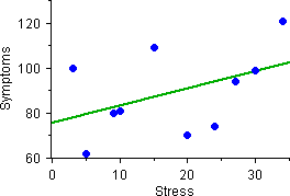As can be seen in the graph to the right, as a college student's stress increases the number of symptoms reported also tends to increase. Each additional point on the stress scale predicts an increase of about .8 symptoms reported. However, the relationship between stress and symptoms is not statistically significant (t(8) = 1.42, r = p = .19). With only ten students, the estimate of the relationship between stress score and number of symptoms is not very accurate. It might be as high as two additional symptoms for each one-unit increase in stress score or it might even be negative--a decrease of .5 symptoms for each one-unit increase in stress score (95-percent confidence interval: [-.48, 2.02]).

Return to Top

Cryer and Miller (1994) on p. 178 present an example of two variables that might be related: a house's size, as measured in hundreds of square feet of living area, and its market value.

Parcel	1	2	3	4	5	6	7	8	9	10
SqFt	5.44	6.94	7.67	8.25	8.99	9.65	10.33	10.60	11.06	12.98
MarketValue	25.2	37.4	33.6	38.0	37.6	37.2	40.4	44.8	42.8	45.2

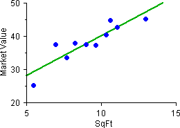As can be seen in the graph to the right, market value increases with the number of square feet of the parcel. For each additional one hundred square feet, the value of the parcel increases by approximately $2,400. While size of parcel and market value are significantly related positively (t(8) = 5.68, r = .895, p = .0005), the estimate of the value of each additional one hundred square feet is not very accurate. It might be as low as $1,420 or as high as $3,360 (95-percent confidence interval: [1.42, 3.36]).

Return to Top

Test	1	2	3	4	5	6	7	8	9	10
Stress	2.5	5	10	15	17.5	20	25	30	35	40
FailTime	63	58	55	61	62	37	38	45	46	19

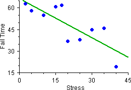As can be seen in the graph to the right, there is a negative relationship between stress applied and the time to failure. Each additional unit of stress (kg/sq mm) significantly decreased failure time by .9 hours or 54 minutes (t(8) = -3.71, r = -.795, p = .006). With only ten observations, the estimate of failure time as a function of stress is not very accurate. Each additional unit of stress (kg/sq mm) might have decreased failure time by only .34 hours or by as much as 1.46 hours (95-percent confidence interval: [-1.46, -.34]).

Return to Top

Ott (1993) presents this example on p. 452: Fifteen male volunteers ate a low-cholesterol diet for four weeks. Below are the ages and the reduction in cholesterol (in mg per 100 ml of blood serum) for each participant:

Participant	1	2	3	4	5	6	7	8	9	10	11	12	13	14	15
Age	45	43	46	49	50	37	34	30	31	26	22	58	60	52	27
Reduce	30	52	45	38	62	55	25	30	40	17	28	44	61	58	45

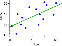As can be seen in the graph to the right, there is a positive relationship between age and the amount of cholesterol reduction achieved by the low-cholesterol diet. For each year older the patient, the diet reduced on average an additional .75 mg of cholesterol per 100 ml of blood serum. While this positive relationship is significant (t(13) = 3.07, r = .65, p = .009), the reduction to be expected is imprecisely estimated. It might be as low as .22 mg or as high as 1.28 mg per 100 ml of blood serum (95-percent confidence interval: [.22, 1.28]).

Return to Top