|| Unconstrained Klein's Model I Example || Constrained Klein's Model I Example ||
Discussion of linear simultaneous equations systems may be found in almost all econometric textbooks. For example, Chapter 18 in Estimation and Inference in Econometrics by Russell Davidson and James G. MacKinnon (ISBN 0-19506011-3, Oxford University Press, 1993), or chapter 19 in Econometric Analysis, 2nd Ed. by William H. Greene (ISBN 0-02-346391-0, Macmillan, 1993).

where Y is an TxK matrix of T observations on K endogenous variables,
X is an TxL matrix of T observations on L exogenous variables, and
 is a KxK matrix of the coefficients
among the endogenous variables, B is an LxK matrix of the coefficients
of the endogenous variables on
the exogenous, and Z is a TxK matrix of unobserved residuals.
Estimates for B and  are found by minimizing the log-likelihood:

where

Not all of the elements of B and  can be estimated. To "identify" the
model it is necessary to fix some elements of B and
  to zero. It is also possible to fix elements of the residual covariance matrix to
zero as well. The diagonal of
  is also fixed
to one as a "normalization". See the references above for details about the
identification of simultaneous models.
Klein's Model I is a well-known example that is presented in many econometrics
textbooks, including the references above. From page 595, Greene (op.cit.)
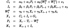
the equations for this model are:
where C is consumption, I investment, Wp private wages, X equilibrium demand,
P private profits, K capital stock, and where
G is government spending, T is indirect business taxes plus net exports,
Wg is the government wage bill, A is time trend measured from 1931.
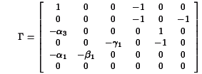
For this model, we get
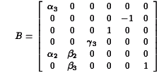
and
and because the last three equations in the model are identities, the last
three columns and rows in the residuals covariance matrix are fixed to zeros.
The program for estimating the coefficients in this model,
klein.prg,is written in the
GAUSS programming language
and uses Aptech System's Maximum Likelihood
(MAXLIK) applications module.
Estimates are produced for a
22 year time series of 9 variables
of the U.S. economy from 1920 through 1941.
The results are presented in klein.out
Klein's Model I is a dynamic model because it contains autoregression coefficients,
i.e., coefficients of endogenous variables on their values at a previous point
in time. For such a model to be dynamically "stable" or stationary, the
model estimates must satisfy a certain condition. Let
For our estimates of Klein's Model I, we have
and
the absolute values of the eigenvalues of which are


 be the submatrix of B associated with the relationships of the endogenous variables
to the exogenous variables that are their lagged versions. Then stability requires
that the eigenvalues of
  be less than
one in absolute value.


  0.0000
  0.0000
  0.0000
  0.0420
  0.4911
  0.4911
This confirms the stability of the model implied by our estimates.
||Top||HomePage||
Greene's book (op.cit.) contains an additional 32 years of data for Klein's Model I. Estimating the model with this additional data presents some difficulties that require the special features of Aptech System's Constrained Maximum Likelihood (CML) applications module.
First, the data are highly correlated, causing difficulty for the estimation process, and second, the unconstrained estimation produces estimates that imply an unstable system.
To deal with the first problem, CML is used to bound the coefficient estimates.
For bounds we will use the 99% confidence limits from the analysis of the
1931 to 1942 data. For the second problem we will use CML to constrain the
eigenvalues of  to be less than one in
absolute value.
The program for estimating the coefficients in this model, cklein.prg,is written in the GAUSS programming language and uses Aptech System's Constrained Maximum Likelihood (CML) applications module.
Estimates are produced for the original 22 year time series of 9 variables of the U.S. economy from 1920 through 1941 plus in addition, the 32 year time series.
The results are presented in klein.out
The results of our stability test are:
  0.0000
  0.0000
  0.0000
  0.0026
  0.9627
  0.9627
The Lagrangean coefficients associated with the constraints on these eigenvalues are:
  0.0000
  0.0000
  0.0000
  1.9556
  0.0000
  0.0000
indicating that the model estimates are on the stability boundary.