Project Summary

In the past, search-type missions have always required a heavy human involvement. Tasks such as monitoring and interpreting sensor readings require extensive operator attention and involvement. In a noisy environment, it becomes difficult for a human operator to classify a sensor reading and quantify confidence in these readings. In this situation, we make use of a probabilistic method to both search for a target and identify anomalies.

The most crucial piece of information required by the ground station is a local magnetic map of the region where the search is taking place. This map of the total magnetic intensity (TMI) of the region may be acquired using analytical models such as the WMM-2000 or WGS-84 model. However, since these models are coefficient-based analytical models, they do not capture temporal or small local variations in magnetic field strength. When an actual search is executed, these small differences between the analytically modeled field and the actual magnetic field will appear as magnetic anomalies. To minimize the number of false anomaly encounters and to increase the accuracy of the simulation and of the search, an actual magnetic survey is used for a local magnetic field map. Data for an actual geomagnetic survey is provided by Fugro Airborne Surveys. The data is collected by a manned aircraft equipped with a magnetometer to measure the total magnetic intensity. This information coupled with a GPS position gives the total magnetic intensity in "line data" form. This data can then be interpolated into a 100x100 meter grid. 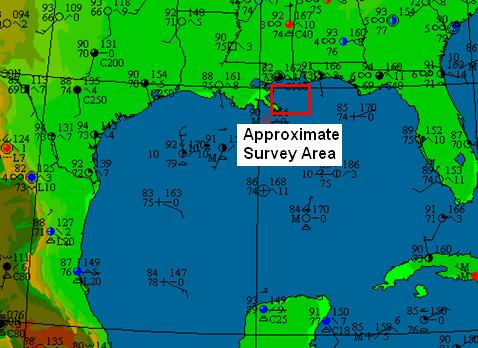Total magnetic intensity readings at locations other than survey points are then linearly interpolated from this square, 100x100 meter grid. The magnetic map and its approximate geographical location are shown below in Figure 1.

Figure 1. Approximate search location and associated total magnetic intensity map

In the above figure, the data is acquired in an approximate 60x50 km grid. The regions of uniform blue denote areas where data is not available. Assuming that there are only permanent fixtures in the region when the map is acquired, this map now makes up the reference set of data on the ground station.

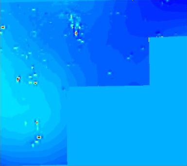
A magnetic model of the desired target is also required. In the following example, we propose a fictional magnetic model of a submarine.

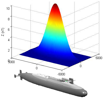
Figure 2. Proposed magnetic signature of submarine

This magnetic signature is a function of many variables, namely sub depth, sensor altitude, etc. Assuming that the magnetic signature of the submarine simply adds to the total magnetic intensity of the local region in a linear fashion, anomalies can easily be identified by simply subtracting the magnetometer reading from the local reference map which is stored on the ground station.

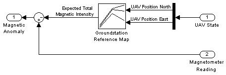
Figure 3. Detecting magnetic anomalies

This architecture shown in Figure 3 can be used to compare magnetometer readings with the reference data to create a differential measurement. Large differential measurements imply the presence of a new magnetic anomaly and possible target. If the UAV does not fly over any targets, the magnetic anomaly should be near zero, excluding small temporal variations in magnetic field and sensor noise. A simple grid search pattern and the associated total magnetic intensity trace and differential measurement trace is shown below in Figure 4.

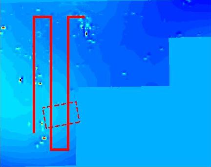
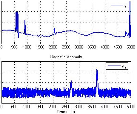
Figure 4. Trajectory and associated sensor measurements

In Figure 4, the location of the target is shown as a dashed red box and the trajectory of the UAV is shown in the solid red line. The total magnetic intensity reading as the UAV flies over this trajectory is shown in the upper trace to the right. The differential measurement is shown in the lower trace.

As the UAV flies this search trajectory, it constantly compares the current sensor reading to the reference data set to create a differential measurement. As can be seen, given the magnetometer reading, it is obvious to detect where the anomaly occurred using the differential measurement even though the actual range of absolute measurements may be large.

As can be seen in Figure 4, one search pattern that can be used is a simple grid search pattern. However, for a team of autonomous agents, a more intelligent approach is desirable. Current research is directed towards employing an occupancy based map search. In this scheme, the search domain is discretized into rectangular grids. Each grid is assigned a score based on the probability that the target is located in that grid. This is similar to a 2 dimensional, discretized probability density function [1]. The initial occupancy map for the domain shown in Figure 1 is shown below in Figure 5.

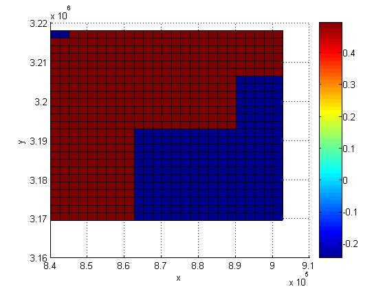
Figure 5. Initial occupancy based map

Here, the cells where no data is available are scored with a zero probability. In effect, this will ensure that the agents only search regions where the total magnetic intensity map is available.

A centralized control structure is used so that the team of autonomous agents can update and formulate control strategies based on a single occupancy map. The basic centralized algorithm that is being used makes use of a team utility function and evolutionary computation ideas. At each sampling period, each agent will assign a score to the cell that is has most recently searched. Once this is complete, each agent evaluates possible control actions from a given population and chooses an appropriate control action which maximizes a given team utility function [2]. This type of behavior is shown below in Figure 6. In this scenario, there are three agents (blue and yellow figures) searching for a single submarine. There are also three false anomalies for them to encounter (brown and red boats).

Figure 6. Agents carrying out search using occupancy map based search

This single map is updated by the agents as they search each grid. If an agent searches a grid and does not encounter any anomalies, this grid is updated with a low score. However, if an agent encounters an anomaly which it then determines to be the target of interest, the immediate grid and several of the surrounding grids are given a high score. This creates a type of gradient that other agents can use to converge on the target. The difficultly arises from accurately and efficiently identifying the encountered anomalies as either the target of interest or as a false anomaly.

Magnetic anomalies can be caused by many factors such as temporal variations in magnetic field or false targets encounters (ie boats/vessels). Once a magnetic anomaly is encountered, it must be identified and classified. In simple terms, the overall goal is to either classify the anomaly as the target or a false reading. Obviously, it would be simple to identify the anomaly if the entire magnetic signature of the anomaly is obtained (ie the UAV flies over the entire boxed region in Figure 4). However, this requires many passes over a potential target. If the anomaly is moving or evading, this may not be possible. The question now becomes, given only one or two passes over the target, is it possible to correctly identify or provide a probability that this anomaly is indeed the target being sough after? To address this issue, a particle filter method is used. This is a non-parametric bayes filter technique which estimates the state of the UAV with respect to the sub using a finite number of state hypotheses.

When the UAV encounters an anomaly whose magnitude exceeds the noise threshold (approximately 1 nT in Figure 4), the particle filter is started in an attempt to estimate the state of the UAV with respect to the target. The particle filter's progression is shown below in Figure 7.

Figure 7. Particle filter progression

In this animation, the large red circle represents the actual location of the UAV. The smaller purple dots represent the particle filter's many different hypotheses of the possible state of the UAV (position north, position east, and heading). This array of state hypotheses are known as particles. As the UAV obtains more and more sensor measurements (at a simulated rate of 1 Hz), the particle filter is able to eliminate particles which are inconsistent with the current measurement and resample these particles to regions which have a higher probability of producing the measured sensor reading. This is why as time progresses, the particles become concentrated about the actual UAV location. Near the end of the simulation, there are four distinct groups of particles. This is due to the symmetry of the underlying target signature. Each of these four groups of particles are equally likely because each group would produce the correct measured sensor readings. Because of this, the particle filter is not able to uniquely identify the position of the UAV with respect to the submarine. This would require multiple passes over the target and more sensor measurements.

Each particle is assigned a weight which is a function of how likely it is to make the correct sensor measurement given its state. For example, a particle which is very close to the actual UAV position has a very high probability that it will make the same projected sensor measurement as the actual UAV, therefore, it is assigned a high score. In contrast, a particle which is farther away from the actual UAV will have a projected measurement which is significantly different from that of the actual UAV and thus, will receive a low score. The sum of all the particle's scores provides a qualitative measure of how confident the particle filter is that the anomaly encountered is the actual target. The sum of the particle weights for an encounter with the actual target and an encounter with a false anomaly is shown below in Figure 8.

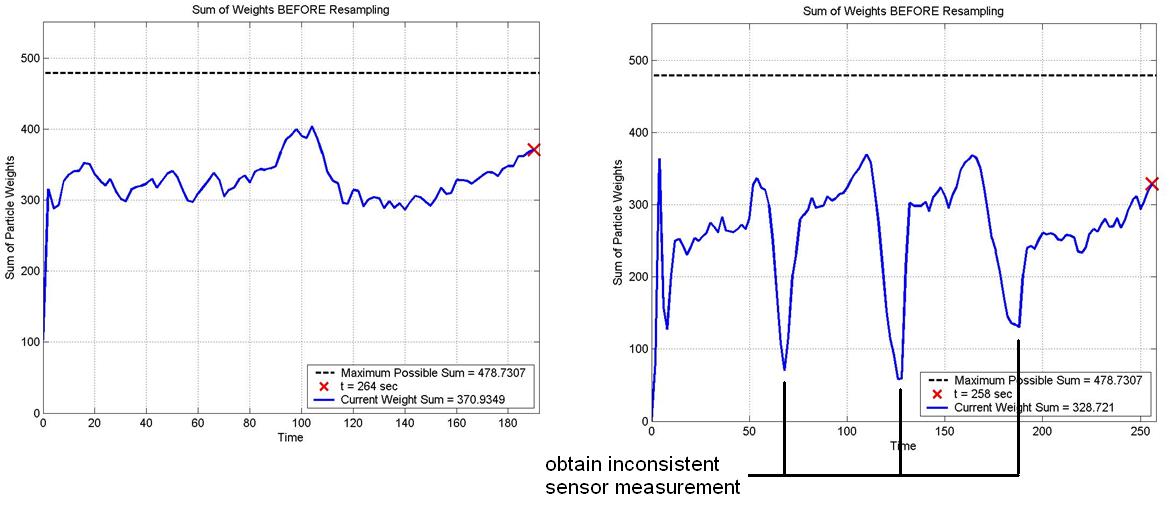
Figure 8. Comparison of sum of weights trace for actual (left) and false (right) anomaly encounter

In Figure 8, the difference between a true target encounter and a false anomaly encounters is fairly clear. In the situation where the UAV encounters the true target, the confidence measure (the sum of all particle weights) increases initially (as the particles are quickly resampled to locations which are consistent with the sensor measurements) and then stays fairly constant. However, in the case where the UAV encounters a false anomaly, the particle filter regularly "loses confidence" as inconsistent sensor measurements are obtained. This is characterized by the sharp drops in the sum of the particle weights. Current research is directed towards training a neural net to recognize these features and thus provide a qualitative measure to the target identification problem. In the end, the particle filter will provide the trace of sum of the weights over time (Figure 8) and the neural net will process this trace. In combination, the particle filter and neural network provides a mapping from magnetic sensor measurements to a single scalar value which represents a measure of how confident the particle filter is that the encountered anomaly is the desired target or not.

References

1. F. Bourgault, T. Furukawa, H.F. Durrant-Whyte, "Coordinated Decentralized Search for a Lost Target in a Bayesian World," Proceedings of the 2003 IEEE/RSJ Intl. Conference on Intelligent Robots and Systems, Las Vegas, Nevada, October 2003.
2. A. Pongpunwattana, "Real-Time Planning for Teams of Autonomous Vehicles in Dynamic Uncertain Environments," Ph.D. Thesis, University of Washington, June, 2004.