CS 261 Lab J - Graph Layouts
Due Wed Nov 26 at 12:00pm
Overview
As we discussed in class, Graphs are a general data structure that can be used for lots of different purposes. One of the interesting features of graphs is that they do not suggest a single spatial layout: the nodes and edges of a graph can be drawn wherever we want without losing any information in the visualization (compare to binary trees, where it mattered whether we drew a branch on the left or right side of its parent!).
Nevertheless, there are certain ways of drawing the graph that are more sensible or aesthetically pleasing: maybe we want to minimize line crossings, or keep similar nodes next to one another. But getting a computer to automatically produce aesthetically pleasing graph visualizations can be quite challenging and algorithmically intensive!
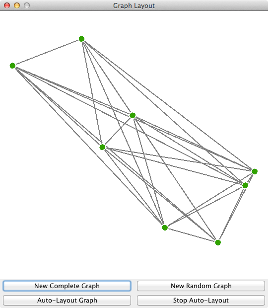
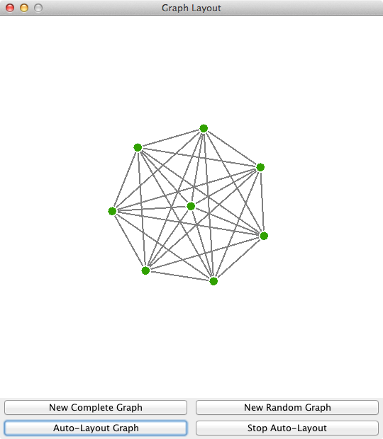
In this lab, you will be implementing a simple force-directed layout algorithm to organize and visualize a randomly generated graph, such that you can take the figure on the left and turn it into the figure on the right:
This lab will be completed in pairs. Partner assignments for this lab can be found on Moodle
- Remember to review the pair programming guidelines before you get started!
Objectives
- To practice working with graphs and get a feel for how connectivity in undirected graphs works.
-
To practice translating and implementing the pseudocode of generic algorithms.
- Turning an algorithm into Java code is an act of translation--and many things can get lost (or gained!) in translation!
- To explore applying physical and mathematical concepts to computer programs
Necessary Files
You will need to download the copy of the GraphLab.zip file. This file contains two classes you will need to import into Eclipse.
-
VisualGraphis an implementation of a simple undirected graph data structure. Each node in this graph does not hold any data, but does have (x,y) coordinates of where it should appear in a visualization. Edges are defined as a pair of nodes (again, without direction or weight).- The inner
NodeandEdgeclasses are placed at the top of the class for your reference. Note that although the instance variables are private, because these are inner classes you can still access them directly. You should not use the getters/setters; those are for other classes! - The inner classes are followed by the instance variables--make sure you know what attributes you have to work with!
- Next is the single method you will have to implement (see instructions below).
- The constructors and other methods are listed last. You won't need to use or modify these, but you're welcome to look at the implementation if you want!
-
Important testing point! The VisualGraph class has a constant called
RANDOM_SEED. This value is used to "start" the random number sequence used to create graphs. If you assign a value that is not 0 to this variable, then your random graphs will always be "random" in the same way. This is very helpful for testing! I recommend assigning a number (e.g., 2) to your graph as you implement the program.
- The inner
-
GraphVisualizationis a regular GUI class that draws a given VisualGraph. Nodes are drawn centered at their (x,y) coordinates, and edges are drawn between these nodes. This class also supports user interaction, in that you can drag nodes around on the screen! Note: you should not modify this class.-
You should start by playing around with the given UI; can you place the nodes in a random graph so that the graph is "aesthetically pleasing"? How did you decide where to place the nodes? Can you translate that into a computer algorithm?
-
Preliminary Information
Force-Directed Layouts
While there are many different algorithms for automatically laying out graphs, this lab will focus on a force-directed layout algorithm. These algorithsm treat the graph as under a set of physical "forces" (think gravity or magnetism) that move the nodes around the graph until they've settled into an equilibrium state--indeed, such algorithms are also known as spring-and-damper algorithms. Because these algorithms model physical forces, we can often borrow simple algorithms from physics such as Columb's Law (the "inverse square law") and Hooke's Law to implement them. You can look at an example force-directed layout (using a different algorithm though) here.
Force-directed layout algorithms are fairly simple to implement, yet produce interesting behaviors and nice layouts. However, they have a bad habit of not being particularly efficient. Because each node influences every other node, they can often be O(n^2) or even O(n^3) (where n may be the number of nodes or edges).
The algorithm you will be implementing works as follows:
- Each node will be treated as a similarly-charged "magnet", so nodes will try and "push" away from each other, moving to opposite sides of the screen
- Each edge will act as a "spring", drawing adjacent (connected) nodes back towards one another.
Thus you can imagine a pair of adjacent nodes as repelling magnets connected by a spring. The magnets will try and push each other away, but eventually the tension of the spring will be greater than the repelling force, so that they won't be able to move further away. The entire graph is treated as a bunch of these magnets connected by springs, and the algorithm involves figuring out how far away everyone wants to be from everyone else, thereby producing a nice graph.
- We apply this algorithm via a loop, like with a simulation---imaging taking a "snapshot" of the forces at work at each individual moment. We calculate the "total force" (all of the repelling from the magnets and attraction from the spring) on all the nodes, and then move them that amount. We then loop and repeat the process, until each node has "settled" into a position where the forces acting on it are about equal.
If you have any questions on this basic idea, please ask for clarification!
As a rough pseucode of the process:
-
//nodes repel each other
for each node 'v'
  for each other node 'u'
    plan to move 'v' away from 'u' based on the distance between them

//edges attract connected nodes
for each edge
  plan to move the two nodes closer to one another based on the distance between them

//actually move the nodes
for each node
  take the amount calculated to move, and apply it to the nodes
  make sure the nodes don't move off the screen
Notes on Vectors
The algorithm you are implementing discusses these physical forces in terms of vectors. If you've never encounted vectors, there is a pretty good introduction here.
The basic idea is that a vector is a pair of numbers that represents a displacement from the current position. For example, the vector (5,2) represents a "move" from the current spot 5 units along the x-axis, and 2 units along the y-axis.
- You can thus thing of each "force" as a vector--so a magnetic repulsion might try to "push" a node in the vector (1.5,-3.5)--or over along the x-axis and down on the y-axis.
Vectors can be added and subtracted--simply add or subtract the x-component and the y-component separately. So (5,2) + (1,2) = (5+1,2+2) = (6,4), and (5,2) - (1,2) = (5-1,2-2) = (4,0). Remember that it is okay for a vector to have a negative component!
- Similarly, this means that if you have a Node at point (100,250), and you have a displacement force of (-35,22), then you can find out where the point should move to by adding the displacement vector:
(100,250) + (-35,22) = (65,272), which would be the new location.
We can also multiply and divide vectors by a scalar--that is, but a single regular number. To do this, simply multiply or divide the x-component and y-component by that number. So (5,2)*3 = (5*3,2*3) = (15,6), and (5,2)/10 = (5/10,2/10) = (0.5,0.2). (We will be working with double-precision vectors!)
- Vector multiplication is more complicated, and we won't be doing any of it here.
Finally, we can also talk about the length or magnitude of a vector. This measures how "long" the displacement is. We write length with a pair of bars around the vector: |v|, where v = (5,2). |v| does not mean the absolute value of the vector! We calculate the length of a displacement by using the distance formula: you can consider the (x,y) pair of the vector as representing it's "end point" when displaced from the origin (0,0), so that the length of the vector is the length of the line from (0,0) to (x,y). Thus \(\mathtt{|(5,2)| = \sqrt{(5-0)^2+(2-0)^2} = 5.385}\).
-
Note that the
Math.hypot(double x, double y)method is a nice, built-in way to find the length of a vector. ThePointclass also has adistance(double px, double py)method that you can use to get the distance of a point (e.g., of a vector) from(0,0). - We can also use the double bar notation to talk about the "size" of a list. For example, |V| could be the "size" of the list of vertices, or the number of vertices in the graph.
Since vectors are represented by a pair of numbers, it makes sense to use a Point object to hold those numbers (though sadly, such objects don't have nice add or subtract methods!) For this lab, we'll be working with vectors in double precision, so you'll want to use the
Point2D.Double
class.
Assignment Details
For this assignment, you will be implementing the Fruchterman-Reingold algorithm. This is one of the simplest and earliest force-directed layout algorithms. It has the benefits of working well on small to medium-sized graphs and converging relatively quickly (within 100 iterations usually). In this model, each node applies a repelling force upon every other node inversely proportional to the square of the distance between them (e.g., like magnetism or gravity). Simpler, edges act as springs that apply an attracting force between nodes that is proportional to the square of the distance between them (again, like magnetism or gravity).
The pseudocode for this algorithm can be found on page 4 of the original paper (and it's really neat to look at the original paper!). The algorithm has also been copied below with some fixed typos for your convenience.
- Note that you will need to make a couple of modifications to this algorithm, described below!
- The pseudocode below is mirrored directly from the paper, since this is how new algorithms are introduced. To do more advanced work in computer science, you'll need to be able to read and process these kinds of algorithms into the programming language and situation (i.e., Java and this lab) that you want.
-
As reported in the paper, this algorithm is
O(\(|V|^2+|E|\)), where |V| is the number of vertices and |E| is the number of edges.
Fruchterman-Reingold Algorithm
1.  area := W * L; { W and L are the width and length of the frame }
2.  G := (V, E); { the vertices are assigned random initial positions }
3.  k := \(\sqrt{area\;/\;|V|}\);
4.  function \(f_a(z)\) := begin return \(z^2 \;/\; k \) end;
5.  function \(f_r(z)\) := begin return \(k^2 \;/\; z \) end;

6.  for i := 1 to iterations do begin
7.      { calculate repulsive forces }
8.      for v in V do begin
9.          { each vertex has two vectors: .pos and .disp }
10.         v.disp := 0;
11.         for u in V do
12.             if (u \(\neq\) v) then begin
13.                 { \(\Delta\) is short hand for the difference vector between the positions of the two vertices }
14.                 \(\Delta\) := v.pos - u.pos;
15.                 v.disp := v.disp + (\(\Delta\;/\;|\Delta|\)) * \(f_r(|\Delta|)\)
16.             end
17.     end

18.     { calculate attractive forces }
19.     for e in E do begin
20.         { each edge is an ordered pair of vertices .v and .u }
21.         \(\Delta\) := e.v.pos - e.u.pos
22.         e.v.disp := e.v.disp - (\(\Delta\;/\;|\Delta|\)) * \(f_a(|\Delta|)\)
23.         e.u.disp := e.u.disp + (\(\Delta\;/\;|\Delta|\)) * \(f_a(|\Delta|)\)
24.     end

25.     { limit the maximum displacement to the temperature i }
26.     { and then prevent from being displaced outside frame }
27.     for v in V do begin
28.         v.pos := v.pos + (v.disp / |v.disp|) * min(|v.disp|, t);
29.         v.pos.x := min(W/2, max(-W/2, v.pos.x));
30.         v.pos.y := min(L/2, max(-L/2, v.pos.y));
31.     end
32.     { reduce the temperature as the layout approaches a better configuration }
33.     t := cool(t);
34. end
This algorithm does not always use the same variable names as the provided class; translating between those variables is part of the assignment!
As stated above, you will have to make a number of modifications to this algorithm to allow it to work with the provided UI system:
- You will need to remove the loop that runs this algorithm through multiple iterations (line 6). The provided GUI includes an animation timer that provides this loop (for infinite iterations); this allows you to see the graph fix its layout in real time, rather than just hitting "go" and getting an organized graph.
-
The "temperature" variable
tis used to slow down the algorithm as it gets into place, as well as to limit the "speed" at which the graph converges into its desired layout (line 28). The smaller this number, the slower the graph will move into place (though its movements will be more precise). I used a value of1.0for this variable, and had thecool()function (line 33) return the same value--that is, the variable started at 1.0 and stayed that way! Others have said a value of 5.0 worked well. You are welcome to experiment with different options and cooling functions.- If you do not provide a cooling function (and you don't have to), your graph should still settle into place. It may seem to "vibrate" in the end (which each node moving one pixel back and forth), but this is expected and acceptable behavior.
-
You will also need to come up with a different method to "
prevent from being displaced outside frame" (line 29-30). For one, our frame goes from (0, 0) to (width, height), not from (-width/2, -height/2) to (width/2, height/2). - You will also want to make it so that the currently "selected" node (e.g., the
excludeparameter in thelayout()method) doesn't get moved. The easiest way to do this is just to not do the final position adjustment on that node (though it should still contribute attractive and repelling forces to other nodes!)
Implementing this algorithm within the provided code and UI is the full extent of this lab! There are a couple of other extensions below however, in case you get done early.
- Note: you may need to "play" with some of the forces and constants to get something that works well for you. Be sure to document any changes you make with comments!
- Try running your algorithm on with bigger and bigger graphs (dozens or hundreds of nodes--you may need to make the window larger!) What do you notice about the algorithm? (hint: think about its Big-O)
- You can continue to drag around nodes as the algorithm runs. Watch the rest of the graph follow your node!
Extensions
As always, there are lots of good extensions you might consider if you have time. You can earn up to 2 points of extra credit for these.
- Add further refinements to the given algorithm. You might add an attractive force at the center of the graph to try and drag nodes away from the walls. You might even give the walls a repelling force.
- Try adding different weights to the nodes and edges. Larger nodes should have more repulsion (and might be drawn larger), and heavier edges might have more attraction (and may be drawn thicker or darker).
- If you're interested, you might look at different algorithms for doing force-directed layouts. Kobourov 2007 (brown.edu) has a nice summary of different options. Implemting the Kamada-Kawai algorithm can be really informative about graphs--you'll need to calculate all-pairs-shortest paths and use some partial derivites, but it can be doable for a motivated student (though not in the time alloted for lab!).
Submitting
Make sure your name is in a class comment at the top of your VisualGraph class and upload all the classes to the LabJ submission folder on vhedwig. Make sure you upload your work to the correct folder! The lab is due at noon on the day after the lab (since we don't have class!)
After you have submitted your solution, log onto Moodle and submit the Lab J Partner Evaluation. Both partners need to submit evaluations.
Grading
This assignment will be graded out of 20 points:
- [5pt] Nodes repulse one another
- [5pt] Edges attract adjacency nodes to one another
- [4pt] Nodes update their position based on the forces applied to them
- [2pt] Nodes stay within the bounds of the screen
- [2pt] Your algorithm lays out the nodes in an aesthetically pleasing fashion (so works overall)
- [1pt] Your algorithms works with the provided UI so that you can see the nodes being re-organized
- [1pt] You have completed your lab partner evaluation